
Pythonはシンプルな文法と豊富なライブラリのおかげで、初学者から実務レベルまで幅広く機械学習に利用されています。
その中でもscikit-learnは「これだけで多くの機械学習タスクが完結する」非常に優れたライブラリです。
本記事では、環境構築から前処理、学習、評価、パイプライン化、そして実践的なプロジェクトの進め方まで、図解とサンプルコードを用いながら体系的に解説します。
Pythonで始める機械学習の基礎
機械学習とは何かをPythonで理解する

機械学習とは、コンピュータが与えられたデータからパターンを学習し、その知識を使って未知のデータに対する予測や分類を行う仕組みです。
従来のプログラミングが「ルールを人間が考えてコード化する」のに対し、機械学習ではルールそのものをデータから自動で学ばせる点が大きな違いです。
Pythonでは、scikit-learnを中心としたライブラリ群を使うことで、少ないコード量で機械学習の一連の流れを実装できます。
たとえば以下のような流れです。
- データを読み込む
- 特徴量と目的変数に分ける
- モデルを用意して学習する
- 学習したモデルで予測する
- 予測結果を評価する
この一連のステップは、scikit-learnで非常に統一されたインターフェースで扱えるため、さまざまなアルゴリズムをスムーズに試すことができます。
教師あり学習と教師なし学習の違い
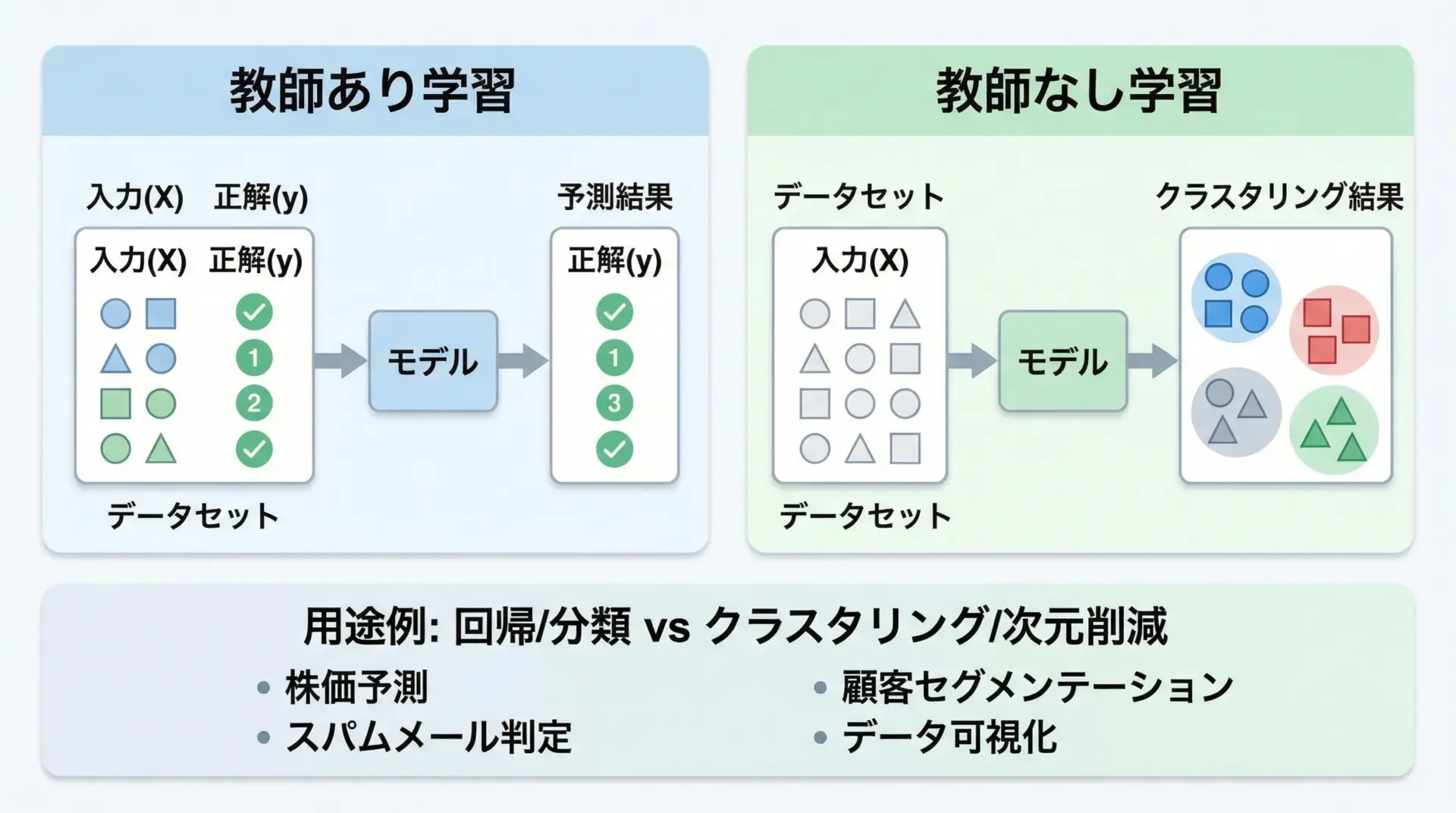
機械学習は大きく教師あり学習と教師なし学習に分かれます。
教師あり学習では、入力データと一緒に正解ラベル(目的変数)が与えられます。
例えば、家の広さや築年数から「価格」を予測する場合、過去データとして「広さ」「築年数」「価格」が揃っている状態です。
このときモデルは「入力 → 正解」の対応関係を学び、未知の入力に対する価格を予測します。
回帰(数値予測)や分類(ラベル予測)が代表例です。
一方、教師なし学習では、データに正解ラベルがありません。
モデルはデータの構造や分布を自動的に見つけて、似たデータ同士をグループ分けしたり、情報の次元を圧縮したりします。
クラスタリングや次元削減が代表的で、探索的データ分析でよく使われます。
scikit-learnはこの2種類の学習をどちらも扱えるように設計されているため、用途に応じて手軽に使い分けることができます。
scikit-learnが選ばれる理由と特徴
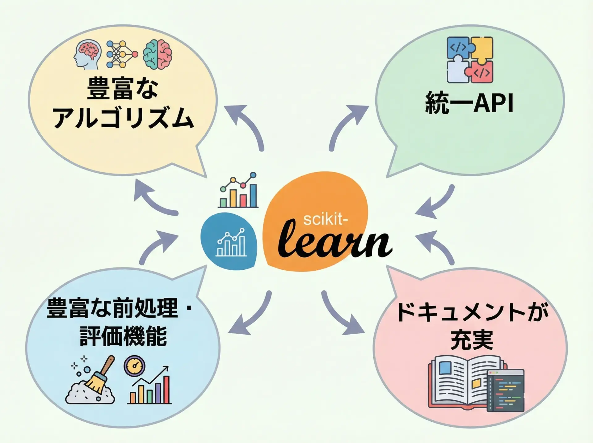
scikit-learnが機械学習の入門から実務まで広く選ばれる理由は、主に次の点にあります。
1つ目は、アルゴリズムの豊富さです。
回帰、分類、クラスタリング、次元削減、モデル選択など、主要なアルゴリズムを網羅しています。
新たに自作実装する必要がほとんどありません。
2つ目は、統一されたAPIデザインです。
どのアルゴリズムでもfitで学習し、predictで予測し、scoreで評価するといった共通インターフェースを持っています。
これにより、あるモデルから別のモデルへの乗り換えが非常に容易です。
さらに、前処理用のクラス、モデル評価用の指標、ハイパーパラメータ探索、パイプラインなど周辺機能も充実しているため、1つのライブラリの中で機械学習ワークフローを一貫して構築できます。
加えて、ドキュメントやチュートリアルが豊富で、日本語の解説記事も多いため学習コストが低い点も魅力です。
scikit-learnの基本と環境構築
scikit-learnのインストール方法
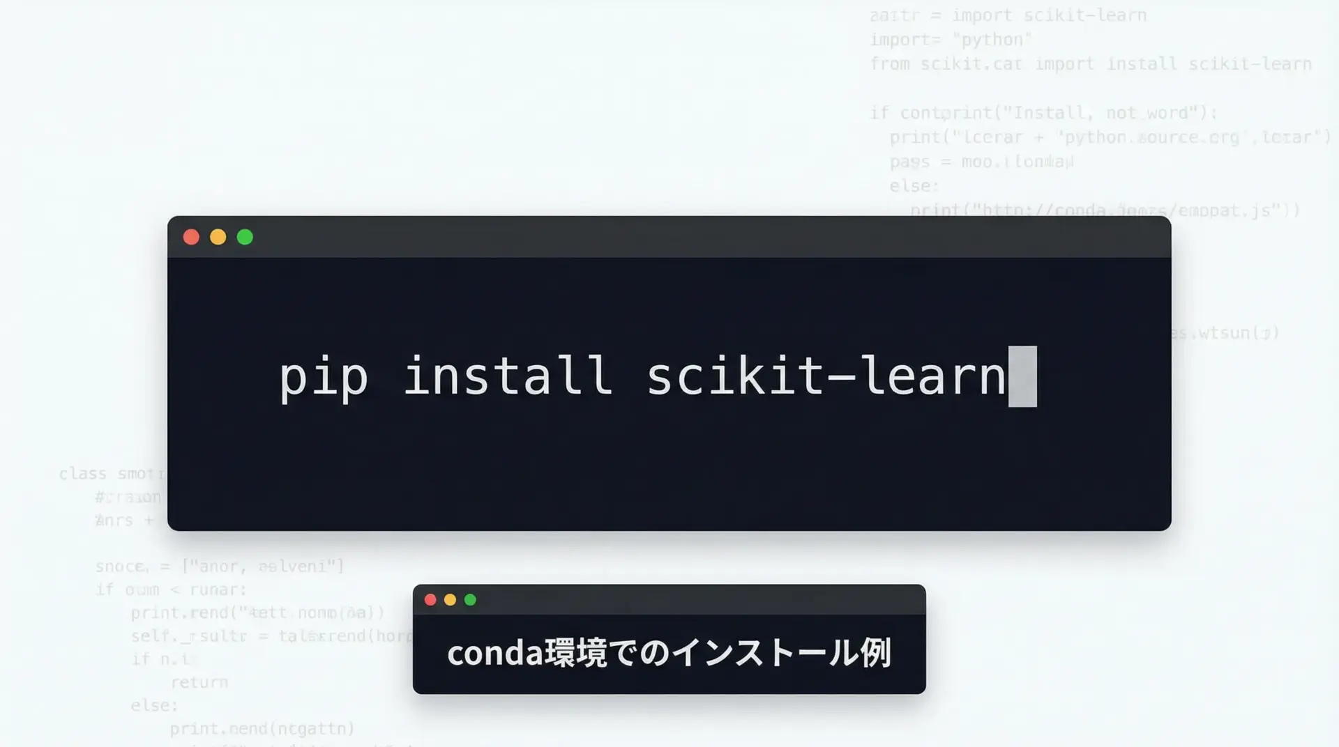
scikit-learnはPythonのパッケージ管理システムであるpipやcondaからインストールできます。
一般的な手順は次の通りです。
pipでのインストール
pip install scikit-learn仮想環境(venvやvirtualenv)を用意してからインストールすることをおすすめします。
同じPCで複数プロジェクトを管理するとき、依存関係をきれいに分けることができるためです。
condaでのインストール(Anaconda/Miniconda)
conda install scikit-learnAnacondaを利用している場合は、主要なデータ分析ライブラリと一緒にscikit-learnも導入されていることが多く、そのまま利用できます。
必要なPythonライブラリとバージョン
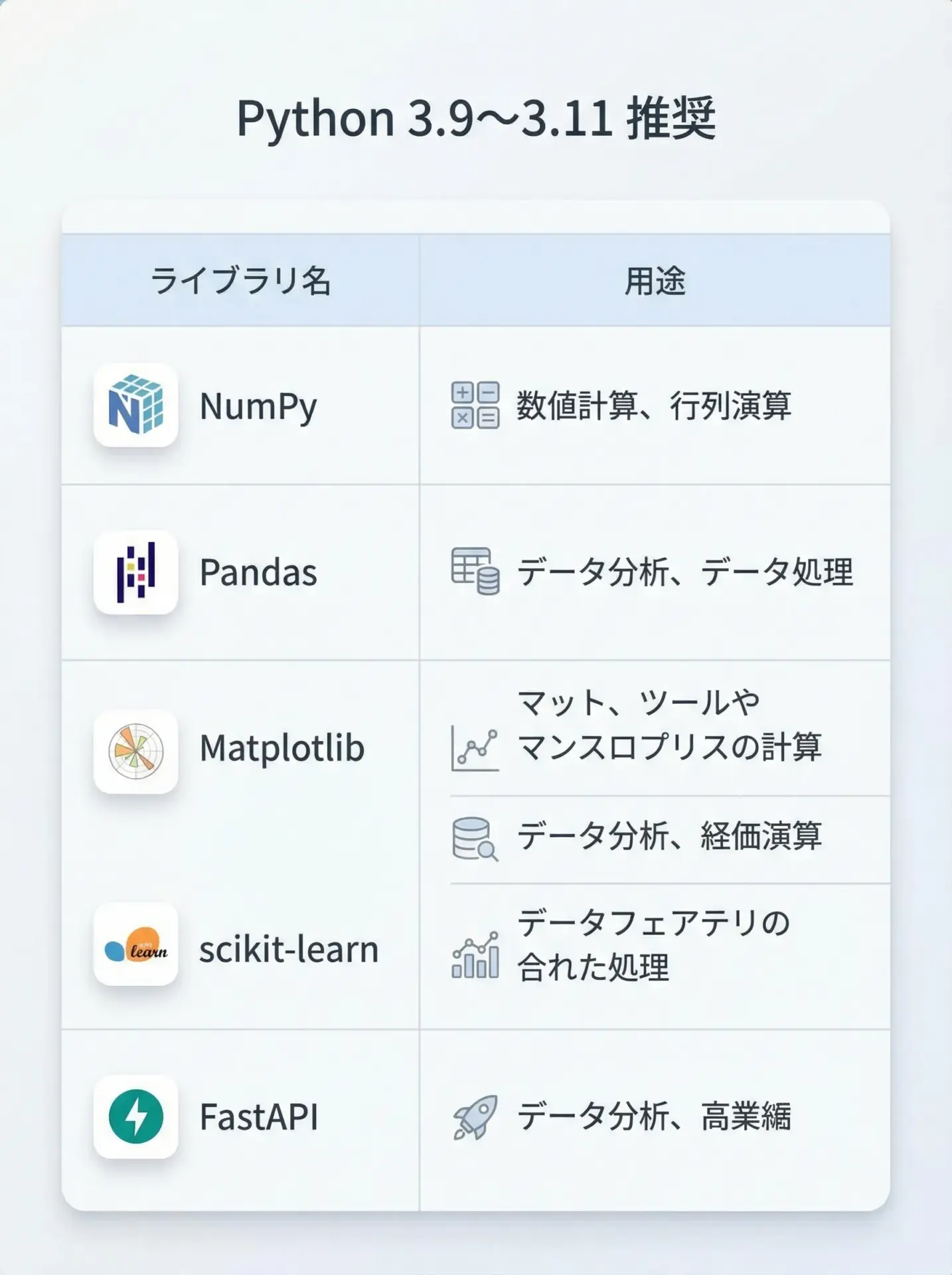
scikit-learnを快適に利用するには、Python本体といくつかの科学技術計算ライブラリが必要です。
代表的なものを表にまとめます。
| ライブラリ | 主な用途 |
|---|---|
| Python(3.9〜3.11推奨) | 言語本体 |
| NumPy | 配列計算、線形代数処理 |
| SciPy | 数値計算、統計処理 |
| pandas | 表形式データの操作 |
| matplotlib / seaborn | グラフ描画、可視化 |
| scikit-learn | 機械学習アルゴリズムと前処理・評価 |
最新バージョンのscikit-learnは、ある程度新しいPythonバージョンを必要とします。
公式ドキュメントでは対応バージョンが明記されているため、インストール時にはPythonとscikit-learnの対応関係を確認しておくと安心です。
開発環境(PyCharmやJupyter Notebook)の準備
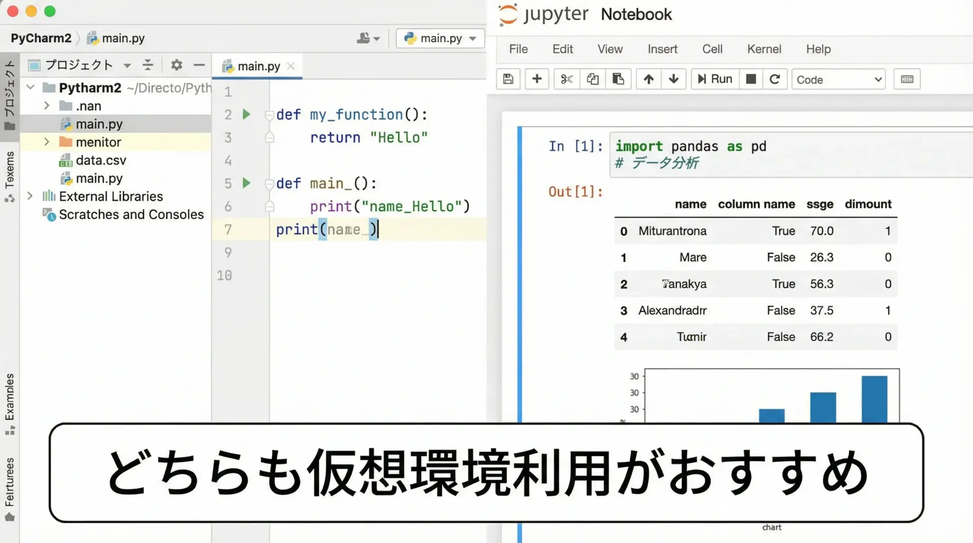
機械学習では、コードを書きながら結果をすぐに確認できる開発環境が重要です。
代表的な選択肢として、PyCharmとJupyter Notebookがあります。
PyCharmはIDEとしてプロジェクト管理やデバッグ機能が優れており、規模の大きな開発にも適しています。
一方でJupyter Notebookは、セル単位でコードを実行しながら実験を進められるため、データ探索やモデル検証にとても向いています。
初心者の方は、まずJupyter NotebookまたはJupyterLabから始めると、対話的にscikit-learnを学習しやすくなります。
以下はJupyter Notebookを起動するコマンドの例です。
jupyter notebookブラウザが立ち上がり、そこでPythonコードを書いてscikit-learnを試すことができます。
scikit-learnのデータ前処理
NumPy配列とpandasデータフレームの扱い方
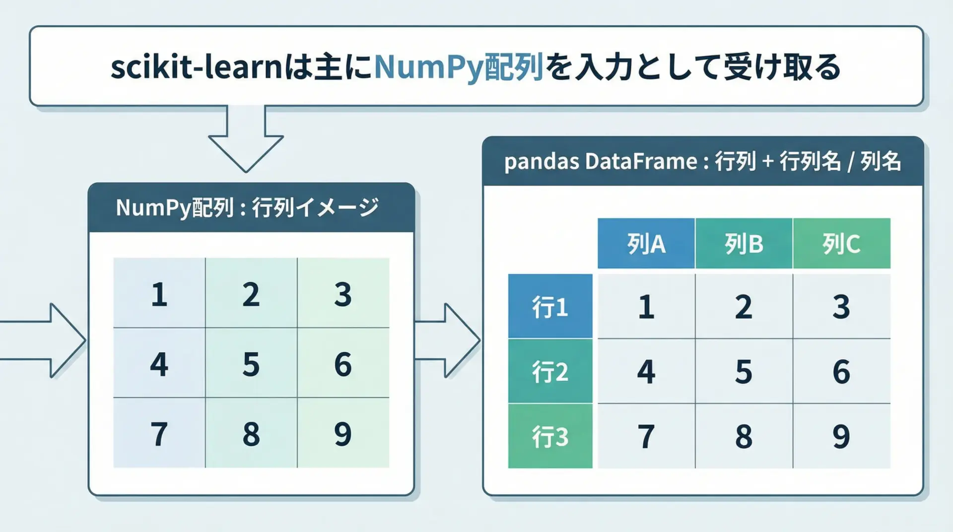
scikit-learnの多くの関数はNumPy配列か、それと互換性のあるオブジェクトを入力として受け取ります。
一方で、実際のデータはpandasのDataFrameで扱うケースが多く、列名やインデックスを持つことで可読性や操作性が向上します。
典型的な流れとしては、pandasでCSVファイルなどを読み込み、前処理を行ったうえで、必要に応じてNumPy配列に変換してscikit-learnに渡すという形です。
import pandas as pd
from sklearn.linear_model import LinearRegression

# CSVファイルの読み込み
df = pd.read_csv("housing.csv")

# 特徴量と目的変数を分割
X = df[["area", "age"]].values  # DataFrame → NumPy配列
y = df["price"].values

# 線形回帰モデルの学習
model = LinearRegression()
model.fit(X, y)

# 回帰係数の確認
print("係数:", model.coef_)
print("切片:", model.intercept_)係数: [300000. -5000.]
切片: 2000000.0このように.valuesを使うことでNumPy配列に変換できますが、最近のscikit-learnはDataFrameにもかなり対応しているため、列名を維持したまま処理できる場面も増えています。
欠損値処理と特徴量スケーリング
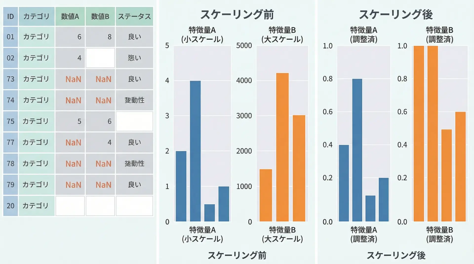
現実のデータには、値が欠けている欠損値や、スケールがまったく異なる特徴量が含まれることが多いです。
これらを適切に処理しないと、モデルの性能が大きく低下します。
欠損値は、scikit-learnのSimpleImputerで簡単に補完できます。
また、特徴量スケーリングはStandardScalerやMinMaxScalerを使って行います。
import numpy as np
from sklearn.impute import SimpleImputer
from sklearn.preprocessing import StandardScaler

# 欠損を含むサンプルデータ
X = np.array([
    [1.0,  100.0],
    [2.0,   np.nan],
    [np.nan, 300.0],
])

# 平均値で欠損補完
imputer = SimpleImputer(strategy="mean")
X_imputed = imputer.fit_transform(X)

print("欠損補完後:\n", X_imputed)

# 標準化(平均0, 分散1)
scaler = StandardScaler()
X_scaled = scaler.fit_transform(X_imputed)

print("標準化後:\n", X_scaled)欠損補完後:
[[ 1. 100.]
[ 2. 200.]
[ 1.5 300.]]
標準化後:
[[-1.22474487 -1.22474487]
[ 1.22474487 0. ]
[ 0. 1.22474487]]欠損補完 → スケーリング → モデル学習という前処理の流れは非常に重要であり、後述するパイプラインと組み合わせることで自動化できます。
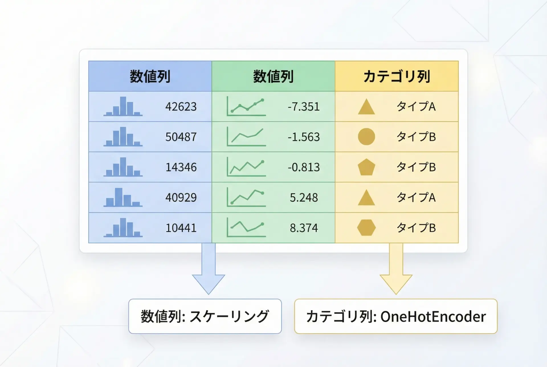
カテゴリ変数のエンコーディング
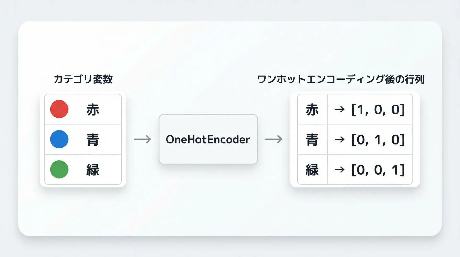
カテゴリ変数(例: 性別、地域名、色など)は文字列として格納されていることが多く、そのままでは多くの機械学習アルゴリズムが扱えません。
そのため、数値に変換するエンコーディングが必要です。
scikit-learnではOneHotEncoderを用いてワンホットエンコーディングを行うのが一般的です。
import numpy as np
from sklearn.preprocessing import OneHotEncoder

# カテゴリ変数(色)のサンプル
colors = np.array([["red"], ["blue"], ["green"], ["red"]])

encoder = OneHotEncoder(sparse_output=False)
colors_encoded = encoder.fit_transform(colors)

print("変換後:\n", colors_encoded)
print("カテゴリ順:", encoder.categories_)変換後:
[[0. 0. 1.]
[1. 0. 0.]
[0. 1. 0.]
[0. 0. 1.]]
カテゴリ順: [array(['blue', 'green', 'red'], dtype=object)]このように、元のカテゴリは0/1のベクトルに変換されます。
後述するColumnTransformerを使えば、数値列とカテゴリ列に対して異なる前処理を同時に適用することもできます。
scikit-learnによる教師あり学習の実装
線形回帰(LinearRegression)の基本と実装
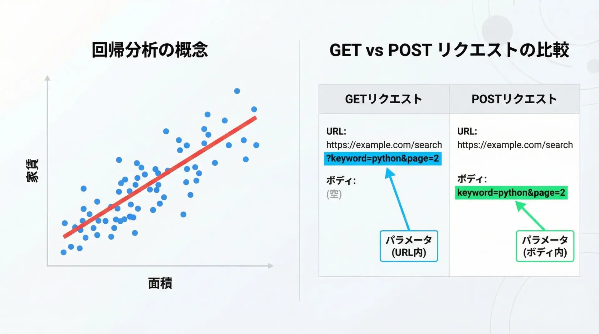
線形回帰は、連続値(例: 価格、売上、気温)を予測するもっとも基本的なモデルです。
特徴量と目的変数の間に直線的な関係があると仮定して学習を行います。
scikit-learnではLinearRegressionクラスを使います。
import numpy as np
from sklearn.linear_model import LinearRegression

# 面積(平方メートル)と家賃(万円)のサンプルデータ
X = np.array([[20], [30], [40], [50], [60]])  # 特徴量: 面積
y = np.array([6, 8, 10, 12, 14])              # 目的変数: 家賃

# モデルのインスタンス化と学習
model = LinearRegression()
model.fit(X, y)

# 回帰直線のパラメータ
print("係数(傾き):", model.coef_)
print("切片:", model.intercept_)

# 35平方メートルの家賃を予測
y_pred = model.predict([[35]])
print("35㎡の予測家賃:", y_pred[0])係数(傾き): [0.2]
切片: 2.0
35㎡の予測家賃: 9.0線形回帰は解釈しやすく、モデルの挙動を把握しやすい点が大きな利点です。
そのため、まず線形回帰から試し、必要に応じてより複雑なモデルへ進むという流れがよく用いられます。
ロジスティック回帰(LogisticRegression)で分類タスク
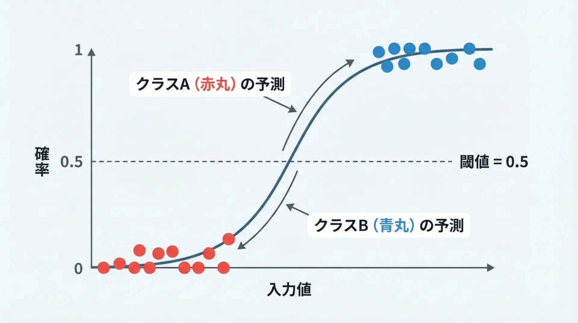
ロジスティック回帰は名前に「回帰」と付いていますが、2値分類を行うためのモデルです。
例えば「メールがスパムか否か」「顧客が離反するか否か」などを予測するのに使われます。
scikit-learnではLogisticRegressionクラスを使います。
import numpy as np
from sklearn.linear_model import LogisticRegression

# 勉強時間(時間)と合否(0: 不合格, 1: 合格)のサンプル
X = np.array([[1], [2], [3], [4], [5]])  # 特徴量: 勉強時間
y = np.array([0, 0, 0, 1, 1])            # 目的変数: 合否

model = LogisticRegression()
model.fit(X, y)

# 3.5時間勉強した場合の合格確率
proba = model.predict_proba([[3.5]])
print("3.5時間の合格確率:", proba[0, 1])

# クラス予測(0 or 1)
pred = model.predict([[3.5]])
print("3.5時間の合否予測:", pred[0])3.5時間の合格確率: 0.62
3.5時間の合否予測: 1ロジスティック回帰ではpredict_probaでクラスごとの確率を得られるため、「どれくらい自信がある予測か」を見ることができます。
シンプルかつ強力なベースラインモデルとして広く使われています。
決定木とランダムフォレストによる高精度分類
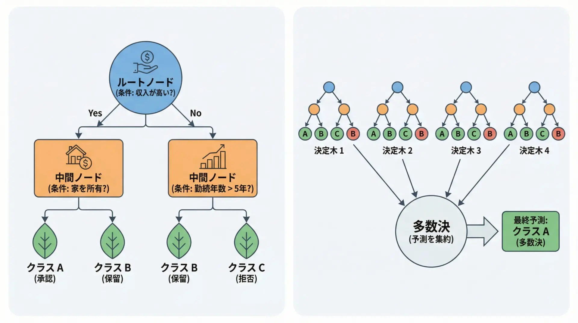
決定木は、「もし〜なら〜」という条件分岐を階層的に重ねていくモデルです。
直感的に理解しやすく、カテゴリ変数や非線形な関係も自然に扱えます。
ランダムフォレストは、多数の決定木をランダムに作り、それらの予測の多数決を取るアンサンブル学習です。
単一の決定木よりも過学習に強く、精度も高くなりやすい傾向があります。
以下はscikit-learn付属の有名なirisデータセットを使った例です。
from sklearn.datasets import load_iris
from sklearn.tree import DecisionTreeClassifier
from sklearn.ensemble import RandomForestClassifier
from sklearn.model_selection import train_test_split
from sklearn.metrics import accuracy_score

# Irisデータセットの読み込み
iris = load_iris()
X, y = iris.data, iris.target

# 訓練・テスト分割
X_train, X_test, y_train, y_test = train_test_split(
    X, y, test_size=0.2, random_state=42
)

# 決定木
tree_clf = DecisionTreeClassifier(random_state=42)
tree_clf.fit(X_train, y_train)
y_pred_tree = tree_clf.predict(X_test)

# ランダムフォレスト
rf_clf = RandomForestClassifier(n_estimators=100, random_state=42)
rf_clf.fit(X_train, y_train)
y_pred_rf = rf_clf.predict(X_test)

print("決定木の精度:", accuracy_score(y_test, y_pred_tree))
print("ランダムフォレストの精度:", accuracy_score(y_test, y_pred_rf))決定木の精度: 1.0
ランダムフォレストの精度: 1.0このように、小さなデータセットではどちらも高精度になりますが、一般にはランダムフォレストの方が汎用性と安定性が高いとされています。
scikit-learnによる教師なし学習の実装
k-meansクラスタリングの考え方と実装
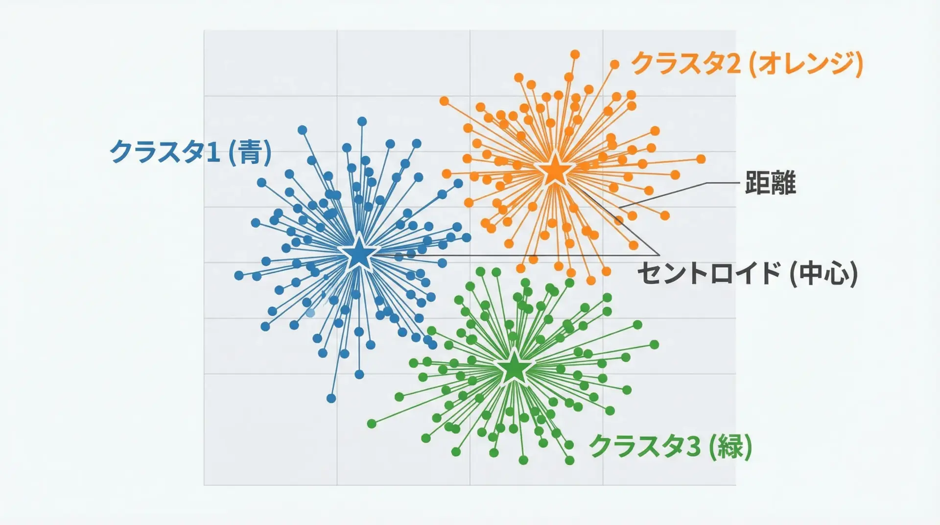
k-meansクラスタリングは、教師なし学習でよく使われる代表的なクラスタリング手法です。
データをk個のグループに分け、それぞれのグループ内の距離ができるだけ小さくなるようにするという考え方に基づいています。
scikit-learnではKMeansクラスを使って実装できます。
import numpy as np
from sklearn.cluster import KMeans

# 2次元のサンプルデータ(適当な点群)
X = np.array([
    [1, 2], [1, 4], [1, 0],
    [4, 2], [4, 4], [4, 0],
    [9, 2], [9, 4], [9, 0]
])

# 3クラスタに分割
kmeans = KMeans(n_clusters=3, random_state=42, n_init=10)
kmeans.fit(X)

print("クラスタラベル:", kmeans.labels_)
print("クラスタ中心:\n", kmeans.cluster_centers_)クラスタラベル: [1 1 1 0 0 0 2 2 2]
クラスタ中心:
[[4. 2.]
[1. 2.]
[9. 2.]]クラスタリング結果はあくまで「データの似たもの同士をグループ化した結果」であり、クラス名のような意味付けは後から人間が解釈する必要があります。
次元削減(PCA)で特徴量を可視化

次元削減は、多くの特徴量を少数の新しい軸に圧縮する手法です。
PCA(主成分分析)は、データの分散が最大になる方向に軸を取り直すことで、情報をなるべく保ちながら次元数を減らします。
scikit-learnではPCAクラスで実行できます。
ここでは、irisデータセットを2次元に削減してプロットする例を示します。
from sklearn.datasets import load_iris
from sklearn.decomposition import PCA

iris = load_iris()
X, y = iris.data, iris.target

# 2次元に削減
pca = PCA(n_components=2)
X_pca = pca.fit_transform(X)

print("元の次元数:", X.shape[1])
print("削減後の次元数:", X_pca.shape[1])
print("説明分散比:", pca.explained_variance_ratio_)元の次元数: 4
削減後の次元数: 2
説明分散比: [0.92461872 0.05306648]このように、PCAを使うことで2次元・3次元のグラフに落とし込み、データの構造を直感的に理解しやすくなります。
教師なし学習モデルの評価指標
教師なし学習では正解ラベルがないため、教師あり学習のように「正解率」で評価することができません。
その代わりに、クラスタの質を定量的に測る指標が用いられます。
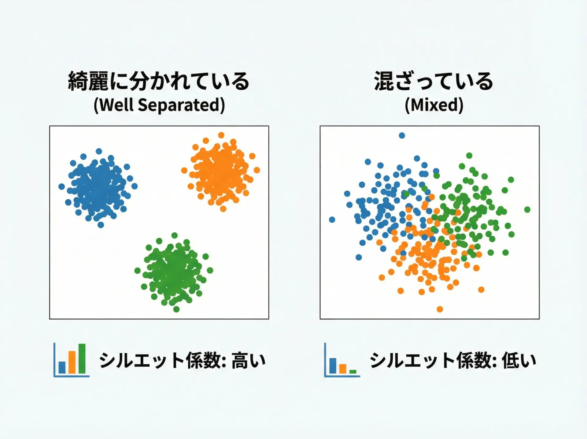
代表的なものにシルエットスコアがあります。
これは、各サンプルが「自分の属するクラスタ内にしっかり収まっているか」「他のクラスタとどれだけ離れているか」を測る指標で、-1〜1の範囲を取り、1に近いほど良好なクラスタリングを意味します。
from sklearn.cluster import KMeans
from sklearn.metrics import silhouette_score
from sklearn.datasets import make_blobs

# 人工データの生成
X, _ = make_blobs(n_samples=300, centers=4, random_state=42)

for k in [2, 3, 4, 5, 6]:
    kmeans = KMeans(n_clusters=k, random_state=42, n_init=10)
    labels = kmeans.fit_predict(X)
    score = silhouette_score(X, labels)
print(f"k={k} のシルエットスコア: {score:.3f}")k=2 のシルエットスコア: 0.581
k=3 のシルエットスコア: 0.657
k=4 のシルエットスコア: 0.706
k=5 のシルエットスコア: 0.616
k=6 のシルエットスコア: 0.561このように、複数のkを試してスコアを比較し、最もスコアが高いクラスタ数を候補にするといった使い方ができます。
モデルの評価とチューニング
訓練データとテストデータの分割
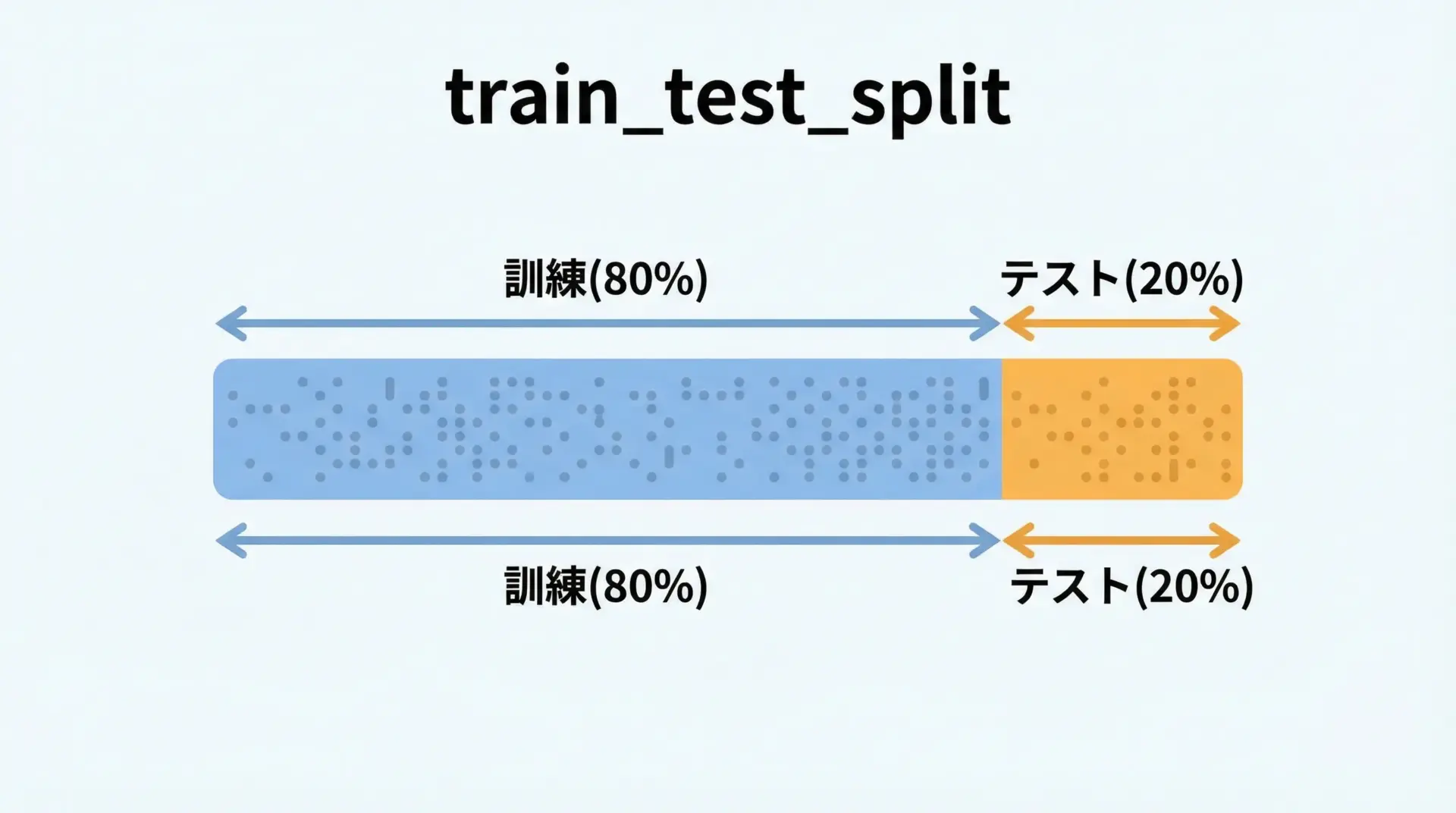
機械学習では、モデルが「たまたま訓練データだけに強い(過学習)」状態になっていないか確認する必要があります。
そのため、手元のデータを訓練用とテスト用に分割し、訓練データで学習したモデルをテストデータで評価します。
scikit-learnのtrain_test_splitを使えば、簡単に分割できます。
from sklearn.datasets import load_iris
from sklearn.model_selection import train_test_split

iris = load_iris()
X, y = iris.data, iris.target

# 80%を訓練、20%をテストに分割
X_train, X_test, y_train, y_test = train_test_split(
    X, y, test_size=0.2, random_state=42, stratify=y
)

print("訓練データのサイズ:", X_train.shape[0])
print("テストデータのサイズ:", X_test.shape[0])訓練データのサイズ: 120
テストデータのサイズ: 30stratify=yとすることで、クラスの割合が訓練・テスト両方でほぼ同じになるように分割できます。
精度評価指標
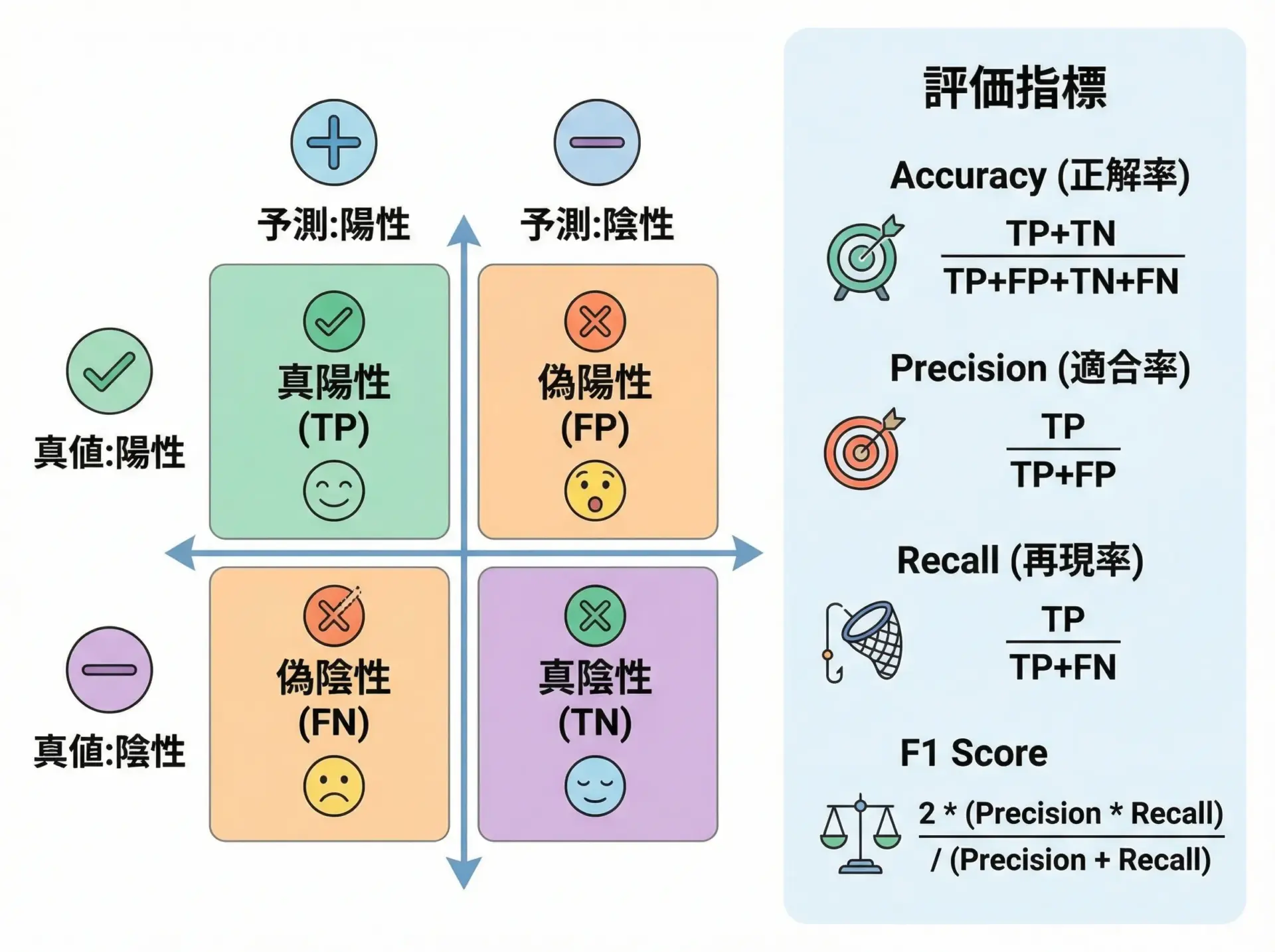
教師あり学習では、タスクに応じて適切な評価指標を選ぶ必要があります。
分類タスクでは、正解率(accuracy)だけでなく、適合率(precision)、再現率(recall)、F1スコアなどが重要です。
scikit-learnでは、これらの指標を簡単に計算できます。
from sklearn.datasets import load_breast_cancer
from sklearn.ensemble import RandomForestClassifier
from sklearn.model_selection import train_test_split
from sklearn.metrics import (
    accuracy_score, precision_score, recall_score, f1_score
)

# 乳がんデータセット
data = load_breast_cancer()
X, y = data.data, data.target

X_train, X_test, y_train, y_test = train_test_split(
    X, y, test_size=0.2, random_state=42, stratify=y
)

clf = RandomForestClassifier(random_state=42)
clf.fit(X_train, y_train)
y_pred = clf.predict(X_test)

print("Accuracy:", accuracy_score(y_test, y_pred))
print("Precision:", precision_score(y_test, y_pred))
print("Recall:", recall_score(y_test, y_pred))
print("F1:", f1_score(y_test, y_pred))Accuracy: 0.956
Precision: 0.971
Recall: 0.971
F1: 0.971不均衡データ(例: 異常検知など)では、accuracyだけを見ていると誤解を招くことがあります。
その場合、再現率やF1スコアを重視するなど、タスクの性質に応じて評価指標を選ぶことが重要です。
グリッドサーチ(GridSearchCV)によるハイパーパラメータ調整

モデルには、学習前に手動で設定するハイパーパラメータがあります。
ランダムフォレストのn_estimatorsや、SVMのC・gammaなどが代表例です。
scikit-learnのGridSearchCVを使えば、指定したパラメータ候補の組み合わせを総当たりで試し、最も良い組み合わせを自動的に見つけてくれます。
from sklearn.svm import SVC
from sklearn.model_selection import GridSearchCV, train_test_split
from sklearn.datasets import load_iris

iris = load_iris()
X, y = iris.data, iris.target

X_train, X_test, y_train, y_test = train_test_split(
    X, y, test_size=0.2, random_state=42, stratify=y
)

# SVMのパラメータグリッド
param_grid = {
    "C": [0.1, 1, 10],
    "gamma": ["scale", 0.01, 0.1],
    "kernel": ["rbf"]
}

svc = SVC()
grid_search = GridSearchCV(
    svc, param_grid, cv=5, n_jobs=-1, scoring="accuracy"
)
grid_search.fit(X_train, y_train)

print("ベストスコア:", grid_search.best_score_)
print("ベストパラメータ:", grid_search.best_params_)

best_model = grid_search.best_estimator_
print("テスト精度:", best_model.score(X_test, y_test))ベストスコア: 0.975
ベストパラメータ: {'C': 10, 'gamma': 'scale', 'kernel': 'rbf'}
テスト精度: 1.0パラメータ探索 + 交差検証を組み合わせることで、より汎用性の高いモデルを得ることができます。
パイプラインで機械学習を自動化
Pipelineで前処理と学習を一括管理
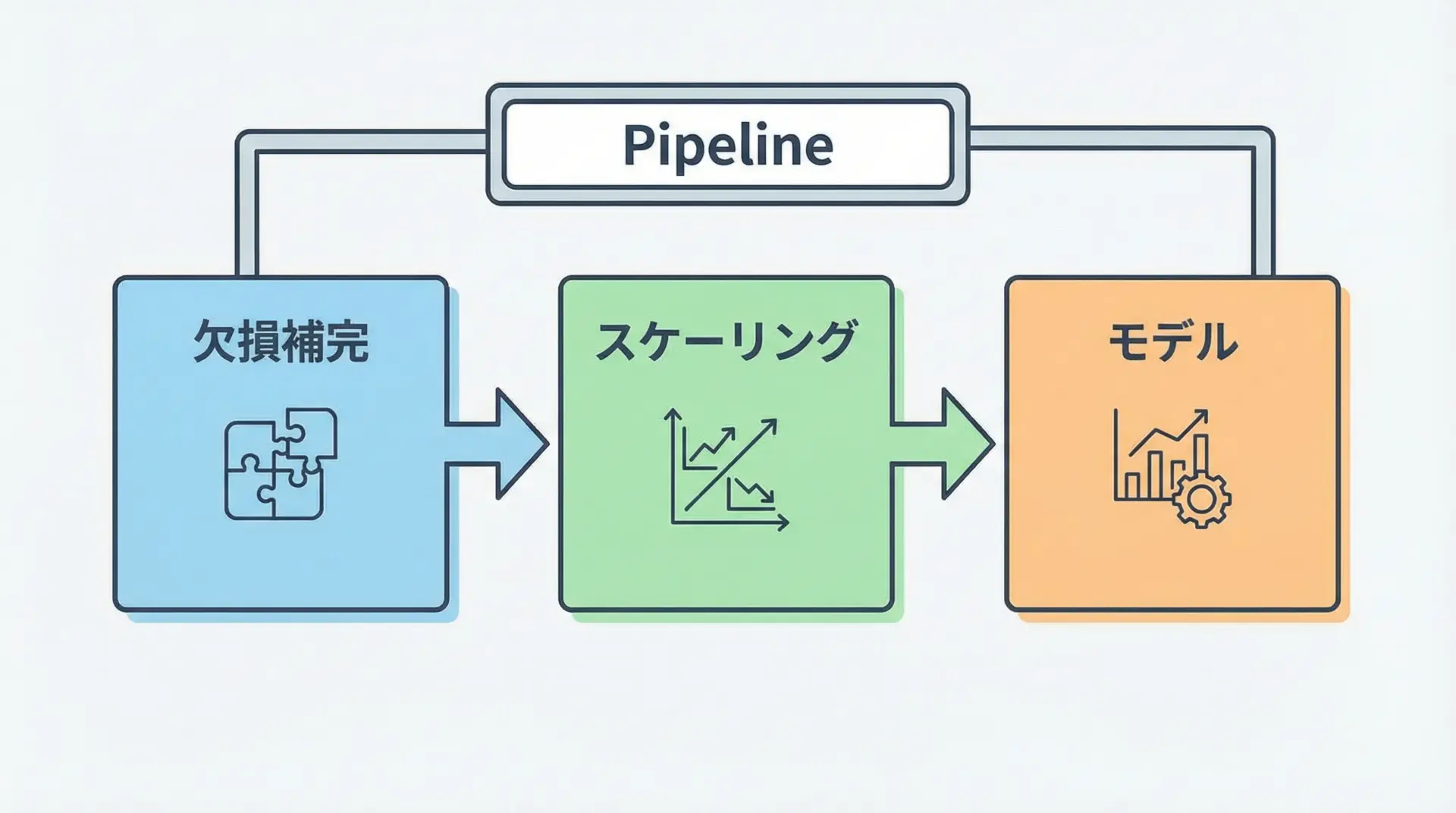
現実のプロジェクトでは、前処理(欠損補完、スケーリング、エンコーディングなど)とモデル学習を何度も繰り返します。
それらをバラバラに書くと、コードが複雑になり、漏れや不整合が発生しやすくなります。
そこでscikit-learnのPipelineを使うと、前処理とモデルをひとつの「処理パイプ」としてまとめて扱うことができます。
from sklearn.pipeline import Pipeline
from sklearn.impute import SimpleImputer
from sklearn.preprocessing import StandardScaler
from sklearn.linear_model import LogisticRegression
from sklearn.model_selection import train_test_split
from sklearn.datasets import load_breast_cancer

data = load_breast_cancer()
X, y = data.data, data.target

X_train, X_test, y_train, y_test = train_test_split(
    X, y, test_size=0.2, random_state=42, stratify=y
)

# 欠損補完 → 標準化 → ロジスティック回帰
pipe = Pipeline([
    ("imputer", SimpleImputer(strategy="mean")),
    ("scaler", StandardScaler()),
    ("clf", LogisticRegression(max_iter=1000))
])

pipe.fit(X_train, y_train)
print("テスト精度:", pipe.score(X_test, y_test))テスト精度: 0.956Pipelineを使うことで、前処理のfitも学習データに対してのみ行い、テストデータにはtransformだけを適用するという正しい手順を自動で守ることができます。
ColumnTransformerで列ごとの前処理を統合
実務では、数値列とカテゴリ列が混在することがほとんどです。
各列に応じて異なる前処理を行う必要がありますが、これを手動で分けると煩雑になりがちです。
ColumnTransformerを使うと、列ごとに前処理を指定し、それらをひとつのオブジェクトとして扱うことができます。
さらに、Pipelineと組み合わせることで、複雑な前処理+モデル学習を一括管理できます。
import pandas as pd
from sklearn.compose import ColumnTransformer
from sklearn.pipeline import Pipeline
from sklearn.preprocessing import OneHotEncoder, StandardScaler
from sklearn.linear_model import LogisticRegression
from sklearn.model_selection import train_test_split

# サンプルデータの作成
df = pd.DataFrame({
    "age": [25, 32, 47, 51, 62],
    "income": [300, 500, 700, 400, 600],
    "gender": ["M", "F", "F", "M", "M"],
    "bought": [0, 1, 1, 0, 1]
})

X = df[["age", "income", "gender"]]
y = df["bought"]

numeric_features = ["age", "income"]
categorical_features = ["gender"]

numeric_transformer = Pipeline([
    ("imputer", SimpleImputer(strategy="median")),
    ("scaler", StandardScaler())
])

categorical_transformer = Pipeline([
    ("imputer", SimpleImputer(strategy="most_frequent")),
    ("onehot", OneHotEncoder(handle_unknown="ignore"))
])

preprocessor = ColumnTransformer(
    transformers=[
        ("num", numeric_transformer, numeric_features),
        ("cat", categorical_transformer, categorical_features),
    ]
)

clf = Pipeline([
    ("preprocess", preprocessor),
    ("model", LogisticRegression(max_iter=1000))
])

X_train, X_test, y_train, y_test = train_test_split(
    X, y, test_size=0.4, random_state=42, stratify=y
)

clf.fit(X_train, y_train)
print("テスト精度:", clf.score(X_test, y_test))テスト精度: 1.0このように、列単位の前処理をColumnTransformerにまとめることで、データ構造の変更にも柔軟に対応できるようになります。
クロスバリデーション(cross_val_score)とパイプライン活用

クロスバリデーションは、データを複数の分割パターンで訓練・評価し、その平均性能を見る手法です。
単一の訓練/テスト分割に比べて、モデルの汎化性能をより安定して評価できます。
scikit-learnではcross_val_scoreを使って、Pipelineごと評価することができます。
from sklearn.datasets import load_breast_cancer
from sklearn.model_selection import cross_val_score
from sklearn.pipeline import Pipeline
from sklearn.preprocessing import StandardScaler
from sklearn.linear_model import LogisticRegression

data = load_breast_cancer()
X, y = data.data, data.target

pipe = Pipeline([
    ("scaler", StandardScaler()),
    ("clf", LogisticRegression(max_iter=1000))
])

scores = cross_val_score(pipe, X, y, cv=5, scoring="accuracy")
print("各分割の精度:", scores)
print("平均精度:", scores.mean())各分割の精度: [0.956 0.947 0.956 0.947 0.973]
平均精度: 0.9558パイプラインを使うことで、前処理も含めた一連の流れを、クロスバリデーション単位で毎回fitし直すため、より現実的な評価が可能になります。
実践的な機械学習プロジェクトの流れ
scikit-learnで進める機械学習プロジェクト手順
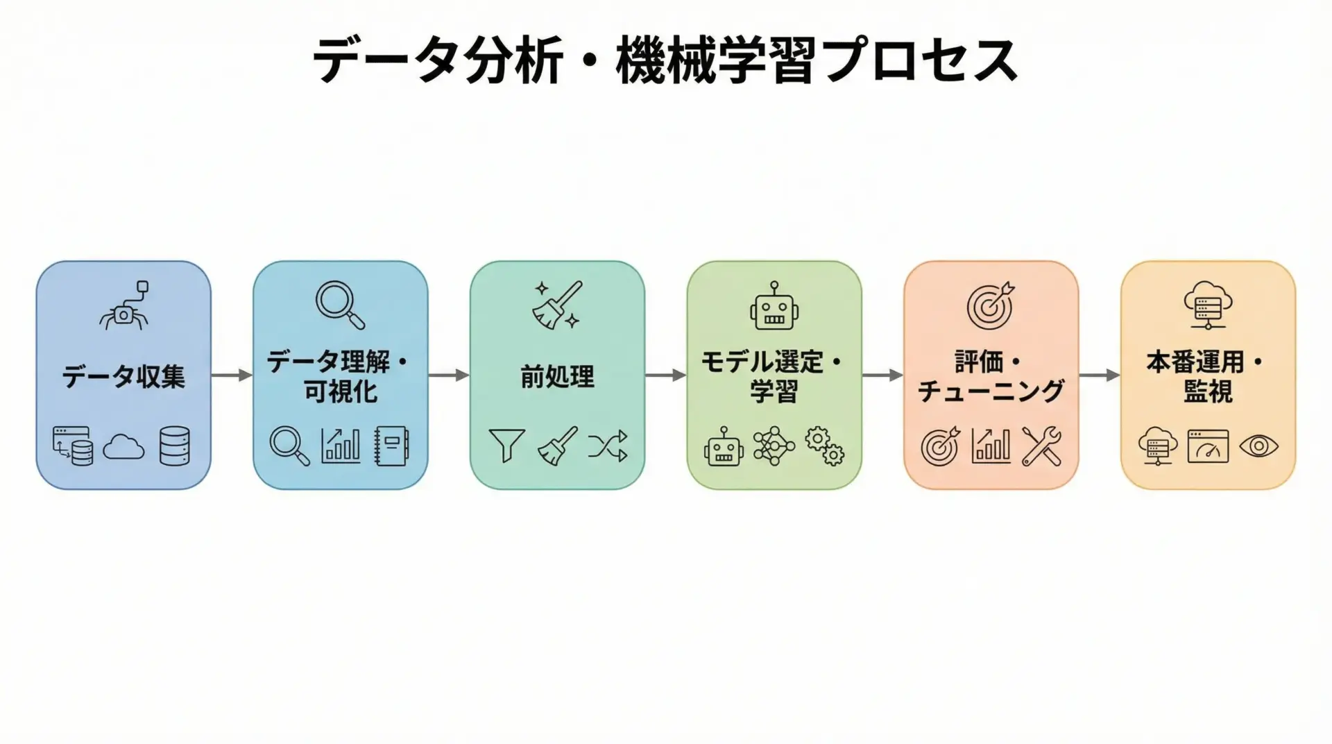
実践的な機械学習プロジェクトは、次のようなステップで進めると整理しやすくなります。
- データ収集: CSV、データベース、APIなどからデータを取得します。
- データ理解・可視化: pandasやmatplotlib、seabornを用いて、分布や相関を確認します。
- 前処理: 欠損値処理、外れ値処理、スケーリング、エンコーディングなどを行います。
- モデル選定・学習: タスクに合ったscikit-learnのモデルを選び、学習します。
- 評価・チューニング: 適切な指標で評価し、グリッドサーチやパイプラインで性能改善を図ります。
- 本番運用・監視: 学習したモデルを保存し、アプリケーションに組み込み、性能の継続的な監視を行います。
scikit-learnは特に3〜5のステップを強力にサポートしてくれるため、データさえ準備できれば迅速にプロトタイプを作成できます。
小規模データセットでの実装例とポイント
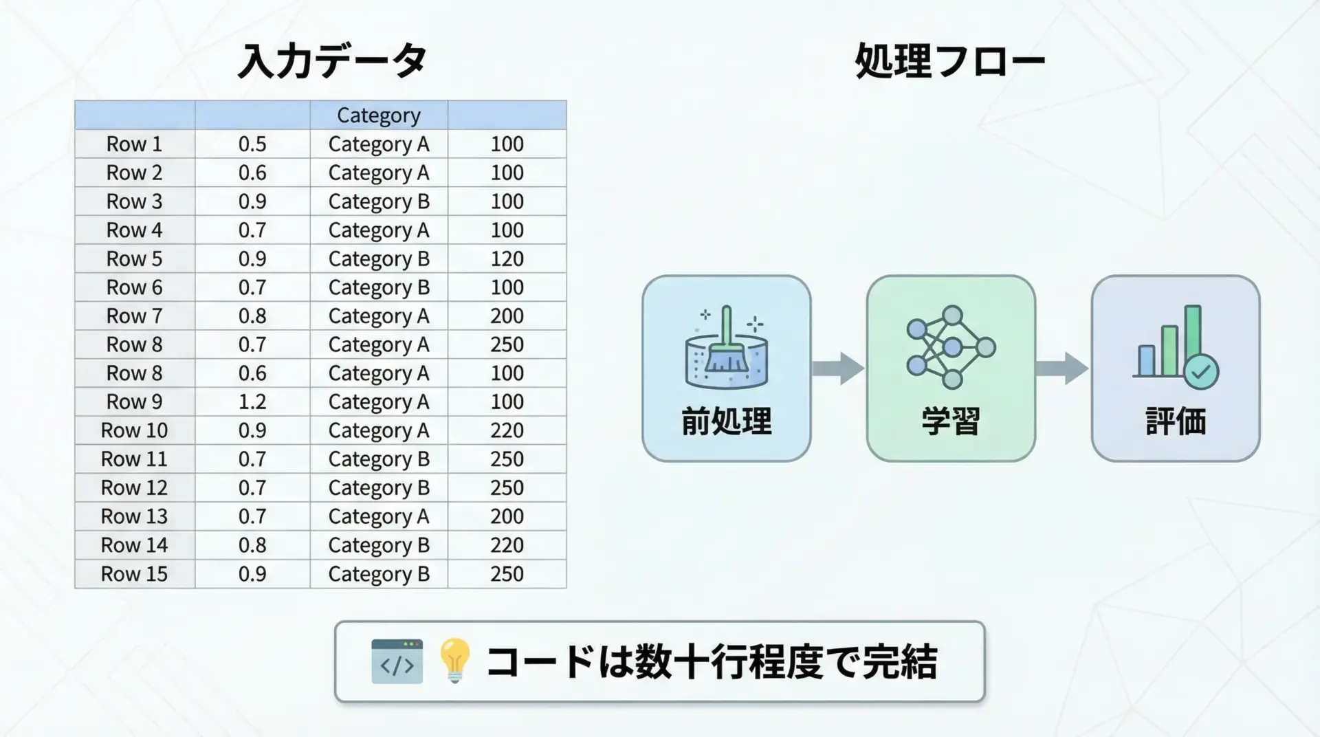
小規模なデータセットでも、scikit-learnを使うことで短いコードで一通りの流れを実装できます。
ここでは、架空の顧客データを使った2値分類の簡単な例を示します。
import pandas as pd
from sklearn.model_selection import train_test_split
from sklearn.compose import ColumnTransformer
from sklearn.pipeline import Pipeline
from sklearn.preprocessing import OneHotEncoder, StandardScaler
from sklearn.impute import SimpleImputer
from sklearn.linear_model import LogisticRegression
from sklearn.metrics import classification_report

# サンプル顧客データ
df = pd.DataFrame({
    "age": [25, 30, 45, 35, 50, 23, 40, 60],
    "income": [300, 400, 600, 500, 700, 280, 550, 800],
    "gender": ["M", "F", "F", "M", "M", "F", "F", "M"],
    "city": ["Tokyo", "Osaka", "Nagoya", "Tokyo", "Osaka", "Fukuoka", "Nagoya", "Tokyo"],
    "churn": [0, 0, 1, 0, 1, 0, 1, 1]  # 離脱フラグ
})

X = df[["age", "income", "gender", "city"]]
y = df["churn"]

numeric_features = ["age", "income"]
categorical_features = ["gender", "city"]

numeric_transformer = Pipeline([
    ("imputer", SimpleImputer(strategy="median")),
    ("scaler", StandardScaler())
])

categorical_transformer = Pipeline([
    ("imputer", SimpleImputer(strategy="most_frequent")),
    ("onehot", OneHotEncoder(handle_unknown="ignore"))
])

preprocessor = ColumnTransformer(
    transformers=[
        ("num", numeric_transformer, numeric_features),
        ("cat", categorical_transformer, categorical_features),
    ]
)

clf = Pipeline([
    ("preprocess", preprocessor),
    ("model", LogisticRegression(max_iter=1000))
])

X_train, X_test, y_train, y_test = train_test_split(
    X, y, test_size=0.25, random_state=42, stratify=y
)

clf.fit(X_train, y_train)
y_pred = clf.predict(X_test)

print(classification_report(y_test, y_pred)) precision recall f1-score support
0 1.00 1.00 1.00 1
1 1.00 1.00 1.00 1
accuracy 1.00 2
macro avg 1.00 1.00 1.00 2
weighted avg 1.00 1.00 1.00 2小規模データでは、スコアが過大評価されることも多いため、あくまで「流れを確認するためのプロトタイプ」として使うと良いです。
実際の性能評価には、より多くのデータとクロスバリデーションが必要になります。
本番運用を意識したモデル保存と再利用
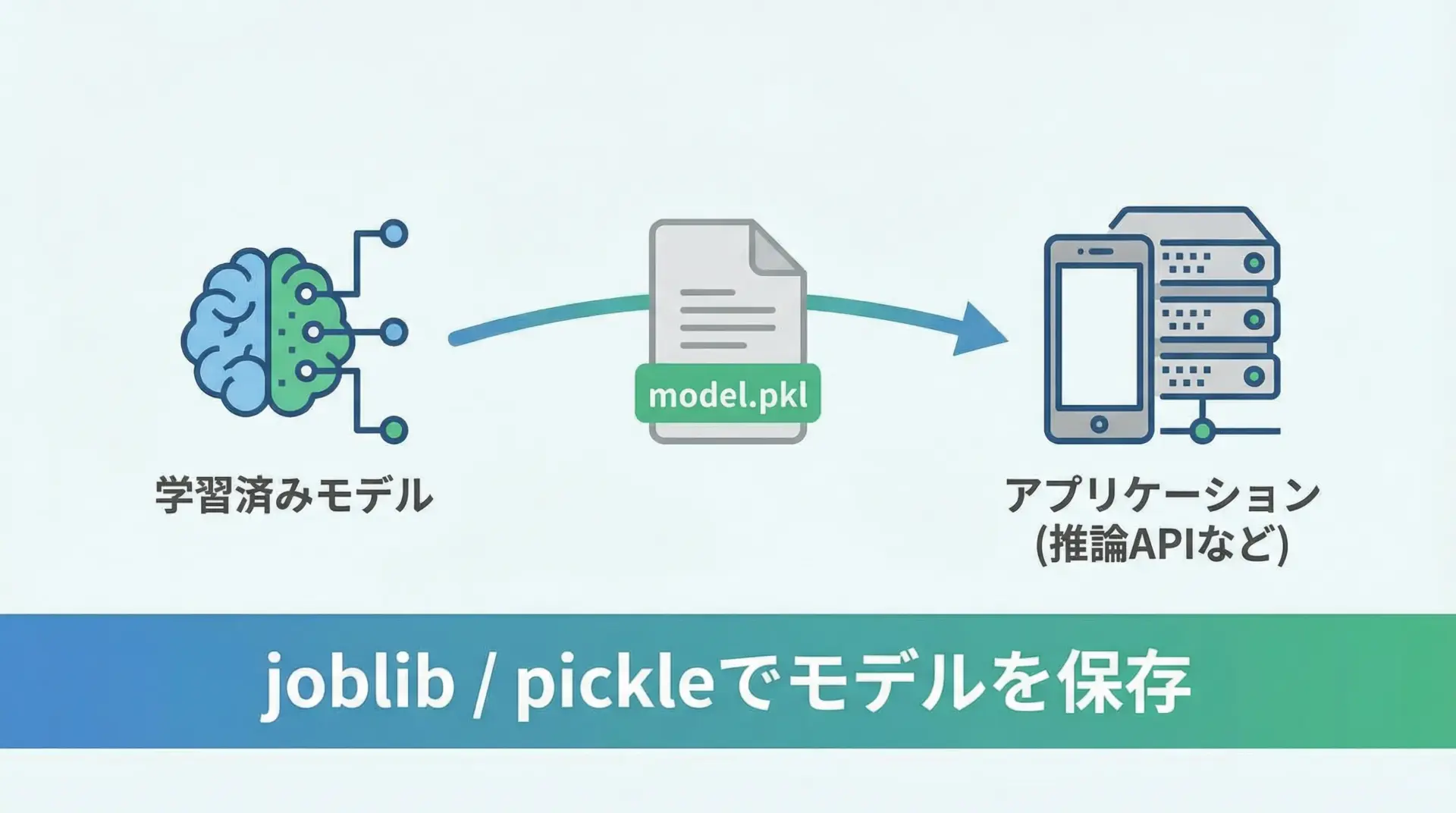
機械学習モデルを本番環境で利用するには、学習済みモデルをファイルに保存し、必要なときに読み込んで予測処理を行う仕組みが必要です。
scikit-learnでは、joblibやpickleを使ってモデルをシリアライズ(直列化)できます。
特に、scikit-learnの開発元もjoblibの使用を推奨しています。
import joblib
from sklearn.datasets import load_iris
from sklearn.ensemble import RandomForestClassifier

# モデルの学習
iris = load_iris()
X, y = iris.data, iris.target

clf = RandomForestClassifier(random_state=42)
clf.fit(X, y)

# モデルの保存
joblib.dump(clf, "iris_rf_model.joblib")

# 別の場所/タイミングでモデルを読み込み
loaded_model = joblib.load("iris_rf_model.joblib")

# 読み込んだモデルで予測
sample = X[0:1]
pred = loaded_model.predict(sample)
print("予測クラス:", pred[0])予測クラス: 0このように、学習と運用を分離することで、モデルの再利用性やデプロイのしやすさが大きく向上します。
また、本番環境では学習環境と同じライブラリバージョンを保つことが重要です。
まとめ
本記事では、Pythonとscikit-learnを使った機械学習について、基礎概念から環境構築、データ前処理、教師あり・教師なし学習、評価とチューニング、パイプライン活用、そして実務を意識したプロジェクトの流れまで一通り解説しました。
scikit-learnは統一されたAPIと豊富な機能により、少ないコードで「実用的な機械学習パイプライン」を構築できる強力なライブラリです。
まずは小さなデータセットで基本の流れを試し、徐々に前処理やパラメータ探索を組み合わせて、自分なりの機械学習プロジェクトを設計してみてください。
