
Pythonでデータ分析や機械学習を行う際に欠かせないのがNumPyです。
NumPyは、多次元配列を中心とした高速な数値計算を可能にするライブラリであり、PandasやSciPy、TensorFlowなど多くのライブラリの基盤にもなっています。
本記事では、NumPyのインストールから配列操作、ブロードキャスト、高速演算、他ライブラリとの連携まで、実務で使えるレベルを目標に体系的かつ丁寧に解説します。
NumPyとは
NumPyがPythonでよく使われる理由
NumPy(ナンパイ)は、Numerical Pythonの略称で、Pythonで数値計算を効率的に行うためのライブラリです。
最大の特徴は多次元配列オブジェクトndarrayを提供し、その上で高速な演算を実現している点にあります。
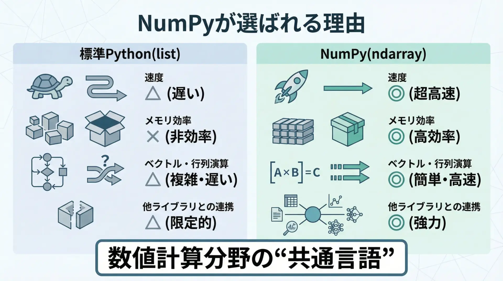
NumPyがよく使われる主な理由は次の通りです。
まず、C言語で実装された内部処理により、標準Pythonのリストに比べて桁違いに高速な数値計算が可能であることが挙げられます。
さらに、配列同士の四則演算、行列積、統計量計算など、数値計算に必要な操作がひと通り揃っているため、複雑な処理を短く直感的なコードで書けます。
また、PandasやSciPy、scikit-learn、TensorFlowなど多くのライブラリがNumPy配列を前提としているため、データ分析・機械学習の基盤技術として必須の存在になっています。
NumPyと標準Python(list)の違い

標準PythonのlistとNumPyのndarrayは、見た目は似ていますが、中身の仕組みが大きく異なります。
listは異なる型のオブジェクトを混在させることができ、その代わりに各要素はポインタ経由で参照されます。
一方、NumPy配列は「同じ型」の値がメモリ上に連続して並んだ構造になっています。
この違いにより、NumPy配列は次のようなメリットを持ちます。
まず、CPUキャッシュが効きやすくなるため、単純な数値演算でも高速化が期待できます。
また、CやFortranなどの低レベル言語から直接アクセスしやすいため、高速なループ処理や線形代数演算をまとめて実行できます。
たとえば、listでベクトルの要素ごとの加算を書こうとすると、forループが必要になりますが、NumPyではa + bのように1行で記述できます。
これはベクトル化(vectorization)と呼ばれ、後述する高速化テクニックの核心でもあります。
NumPyのインストールと環境構築
pipでのNumPyインストール方法
まずはNumPyをインストールする方法を確認します。
一般的なPython環境であれば、pipコマンドから簡単に導入できます。
# NumPyをインストール
pip install numpy

# 既にインストールされている場合はアップグレード
pip install --upgrade numpy
Windows、macOS、Linuxいずれでも、基本的には同じコマンドでインストールできます。
企業環境などでプロキシ越しの接続が必要な場合は、--proxyオプションを使うこともあります。
インストール後、Pythonインタプリタで次のように入力し、エラーが出なければ導入成功です。
import numpy as np
print(np.__version__)
仮想環境でのNumPy導入手順

実務では、プロジェクトごとに依存パッケージのバージョンが異なることがよくあります。
そのため、仮想環境を作成し、その中にNumPyをインストールする運用が推奨されます。
ここでは標準のvenvモジュールを例に説明します。
# 1. 仮想環境の作成 (envという名前の環境を作る例)
python -m venv env

# 2. 仮想環境の有効化
# Windows (PowerShell)
env\Scripts\Activate.ps1

# macOS / Linux (bash, zsh など)
source env/bin/activate

# 3. 仮想環境内にNumPyをインストール
pip install numpy

# 4. 作業が終わったら仮想環境を終了
deactivate
仮想環境を使うことで、あるプロジェクトAではNumPy 1.26系、別のプロジェクトBではNumPy 2.x系というように、バージョン違いを安全に共存させることができます。
NumPy配列(ndarray)の基本
ndarrayの特徴とメリット

NumPy配列ndarrayは、NumPyの核となるデータ構造です。
特徴を整理すると次のようになります。
まず、任意次元の配列を表現できることが重要です。
1次元のベクトルだけでなく、2次元の行列、3次元以上のテンソルも同じインターフェースで扱えます。
また、前述の通り配列の全要素は同じ型で統一されているため、メモリ効率がよく、数値演算が高速に実行されます。
さらに、ブロードキャストと呼ばれる仕組みにより、形状の異なる配列同士でも、一定のルールのもとで自動的に次元が調整され、直感的な演算が可能です。
この性質により、複雑なforループを書かなくても、短いコードで大規模データを処理できます。
リストからNumPy配列を作成する方法
NumPy配列は、Pythonのリストやタプルから簡単に作成できます。
もっとも基本的な関数はnp.arrayです。
import numpy as np

# Pythonのリスト
py_list = [1, 2, 3, 4, 5]

# リストからNumPy配列(ndarray)を作成
arr = np.array(py_list)

print("Pythonリスト:", py_list)
print("NumPy配列:", arr)
print("型:", type(arr))Pythonリスト: [1, 2, 3, 4, 5]
NumPy配列: [1 2 3 4 5]
型: <class 'numpy.ndarray'>多次元データの場合も、入れ子のリストからそのまま配列を生成できます。
# 2次元リストから2次元配列(行列)を作る
py_list_2d = [[1, 2, 3],
              [4, 5, 6]]

arr_2d = np.array(py_list_2d)

print("2次元配列:\n", arr_2d)2次元配列:
[[1 2 3]
[4 5 6]]配列の形状(shape)と次元(ndim)を確認する
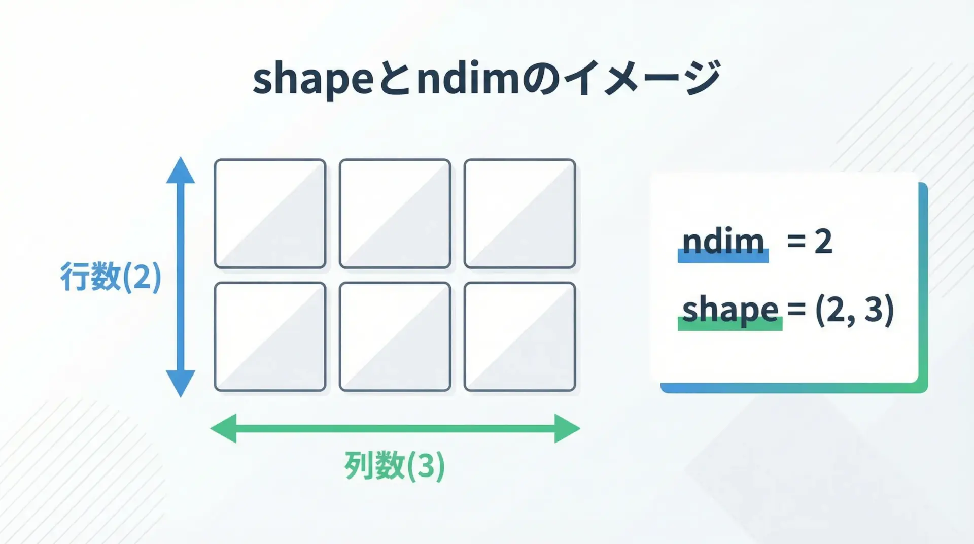
NumPy配列を扱う上で、shape(形状)とndim(次元数)の理解は必須です。
これらは属性として簡単に確認できます。
import numpy as np

arr_1d = np.array([1, 2, 3, 4])
arr_2d = np.array([[1, 2, 3],
                   [4, 5, 6]])

print("1次元配列 shape:", arr_1d.shape, "ndim:", arr_1d.ndim)
print("2次元配列 shape:", arr_2d.shape, "ndim:", arr_2d.ndim)1次元配列 shape: (4,) ndim: 1
2次元配列 shape: (2, 3) ndim: 2shapeは各次元のサイズをタプルで返します。
ndimは配列が何次元かを整数で表します。
この2つを意識しておくと、後述するブロードキャストや線形代数計算の理解が大きく進みます。
NumPy配列の生成と初期化
arangeとlinspaceで数列配列を作る
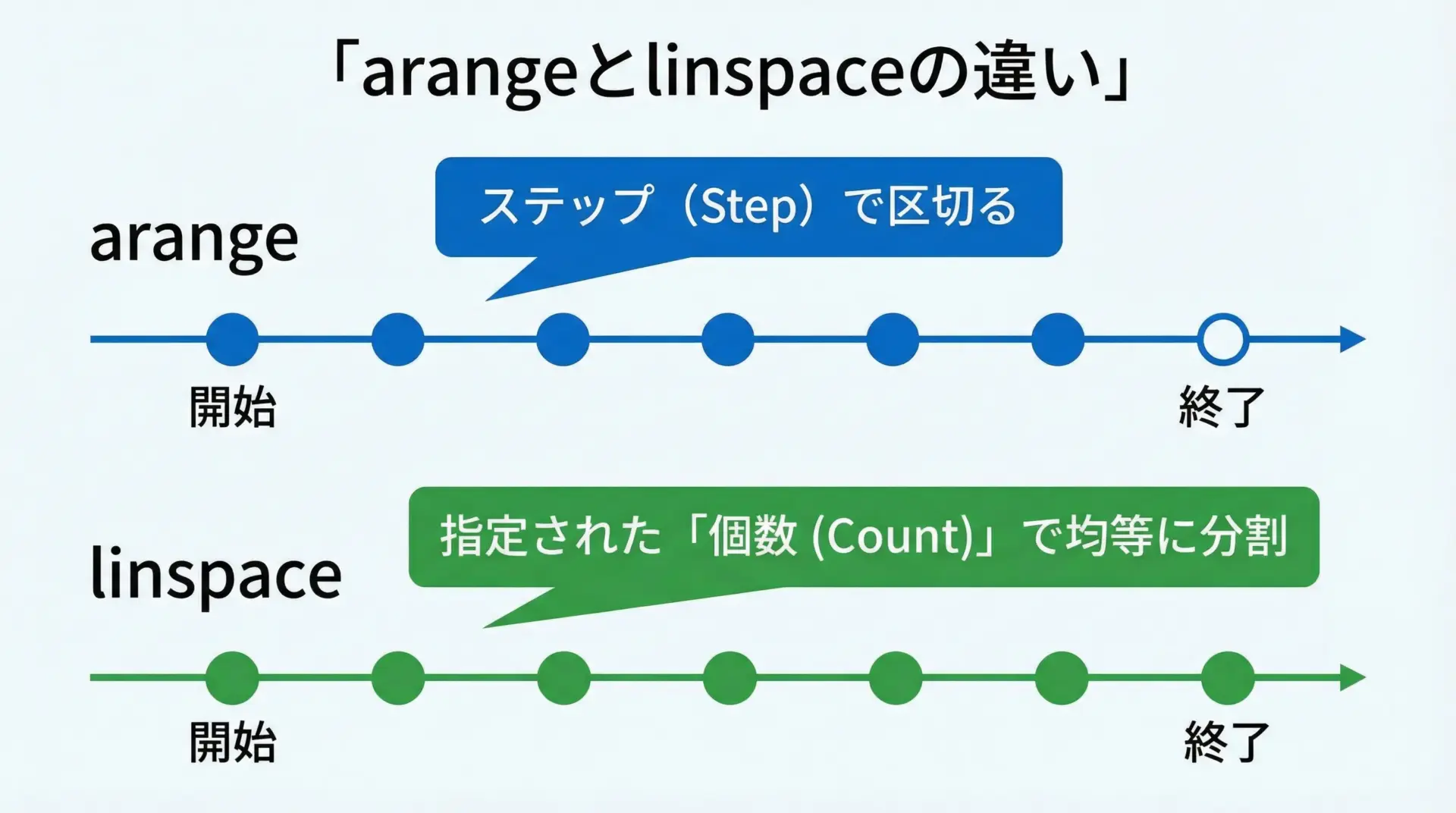
連番の配列を作るときによく使われるのがnp.arangeとnp.linspaceです。
import numpy as np

# arange(開始, 終了, ステップ)
arr1 = np.arange(0, 10, 2)  # 0, 2, 4, 6, 8

# linspace(開始, 終了, 個数)
arr2 = np.linspace(0, 1, 5)  # 0.0 〜 1.0 を5分割

print("arange:", arr1)
print("linspace:", arr2)arange: [0 2 4 6 8]
linspace: [0. 0.25 0.5 0.75 1. ]arangeはステップ幅を指定して区間を刻むため、整数の連番などに便利です。
一方、linspaceは開始から終了までを指定した個数で等間隔に区切るため、グラフ描画用の連続値などに適しています。
zeros・ones・fullで初期化配列を作る
配列をあらかじめ特定の値で埋めておきたい場合は、zeros、ones、fullが便利です。
import numpy as np

# 要素がすべて0の配列
z = np.zeros((2, 3))    # 2行3列

# 要素がすべて1の配列
o = np.ones((2, 3))     # 2行3列

# 要素がすべて7の配列
f = np.full((2, 3), 7)  # 2行3列を7で埋める

print("zeros:\n", z)
print("ones:\n", o)
print("full:\n", f)zeros:
[[0. 0. 0.]
[0. 0. 0.]]
ones:
[[1. 1. 1.]
[1. 1. 1.]]
full:
[[7 7 7]
[7 7 7]]これらの関数は、ニューラルネットワークの重みの初期化や、一時的なバッファ配列の確保などに頻出します。
randomで乱数配列を生成する
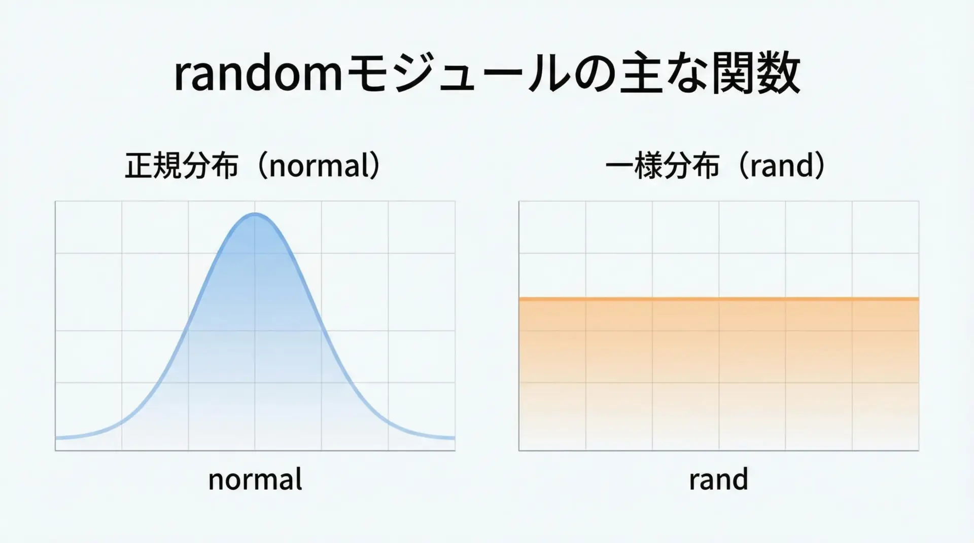
NumPyには乱数生成のためのnp.randomモジュールが用意されています。
代表的な使い方をいくつか紹介します。
import numpy as np

# 0以上1未満の一様乱数 (2行3列)
u = np.random.rand(2, 3)

# 標準正規分布(平均0, 分散1)に従う乱数 (2行3列)
n = np.random.randn(2, 3)

# 指定した範囲の整数乱数 [low, high)
i = np.random.randint(0, 10, size=(2, 3))

print("一様乱数:\n", u)
print("正規乱数:\n", n)
print("整数乱数:\n", i)一様乱数:
[[0.49 ...]
[... ]]
正規乱数:
[[-0.21 ...]
[... ]]
整数乱数:
[[3 8 0]
[1 9 4]]シミュレーションや機械学習のパラメータ初期化など、乱数は実務でも頻繁に利用されます。
再現性を保ちたい場合は、np.random.seed(0)で乱数シードを固定しておくとよいです。
NumPy配列のインデックスとスライス
基本的なインデックス指定とスライス
NumPy配列は、Pythonのリストと同様のインデックス・スライス構文をサポートしています。
import numpy as np
arr = np.arange(10) # [0 1 2 3 4 5 6 7 8 9]
print("arr:", arr)
print("先頭要素:", arr[0])
print("末尾要素:", arr[-1])
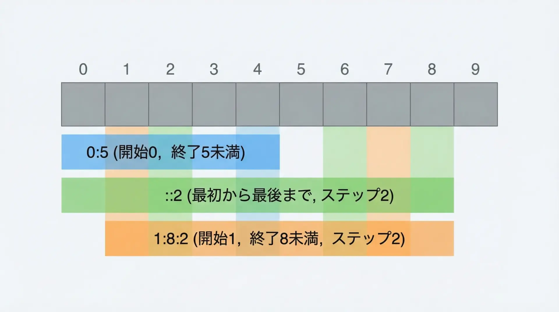
print("0〜4番目:", arr[0:5]) # 0〜4
print("偶数番目のみ:", arr[::2]) # ステップ2arr: [0 1 2 3 4 5 6 7 8 9]
先頭要素: 0
末尾要素: 9
0〜4番目: [0 1 2 3 4]
偶数番目のみ: [0 2 4 6 8]2次元配列の場合は、行と列をカンマで区切って指定します。
import numpy as np

mat = np.arange(1, 13).reshape(3, 4)
print("行列:\n", mat)

# 単一要素
print("要素(1行2列):", mat[0, 1])       # 1行目2列目(0始まり)

# 行のスライス
print("1〜2行目すべての列:\n", mat[0:2, :])

# 列のスライス
print("全行の2〜3列目:\n", mat[:, 1:3])行列:
[[ 1 2 3 4]
[ 5 6 7 8]
[ 9 10 11 12]]
要素(1行2列): 2
1〜2行目すべての列:
[[1 2 3 4]
[5 6 7 8]]
全行の2〜3列目:
[[ 2 3]
[ 6 7]
[10 11]]ブールインデックスで条件抽出する方法
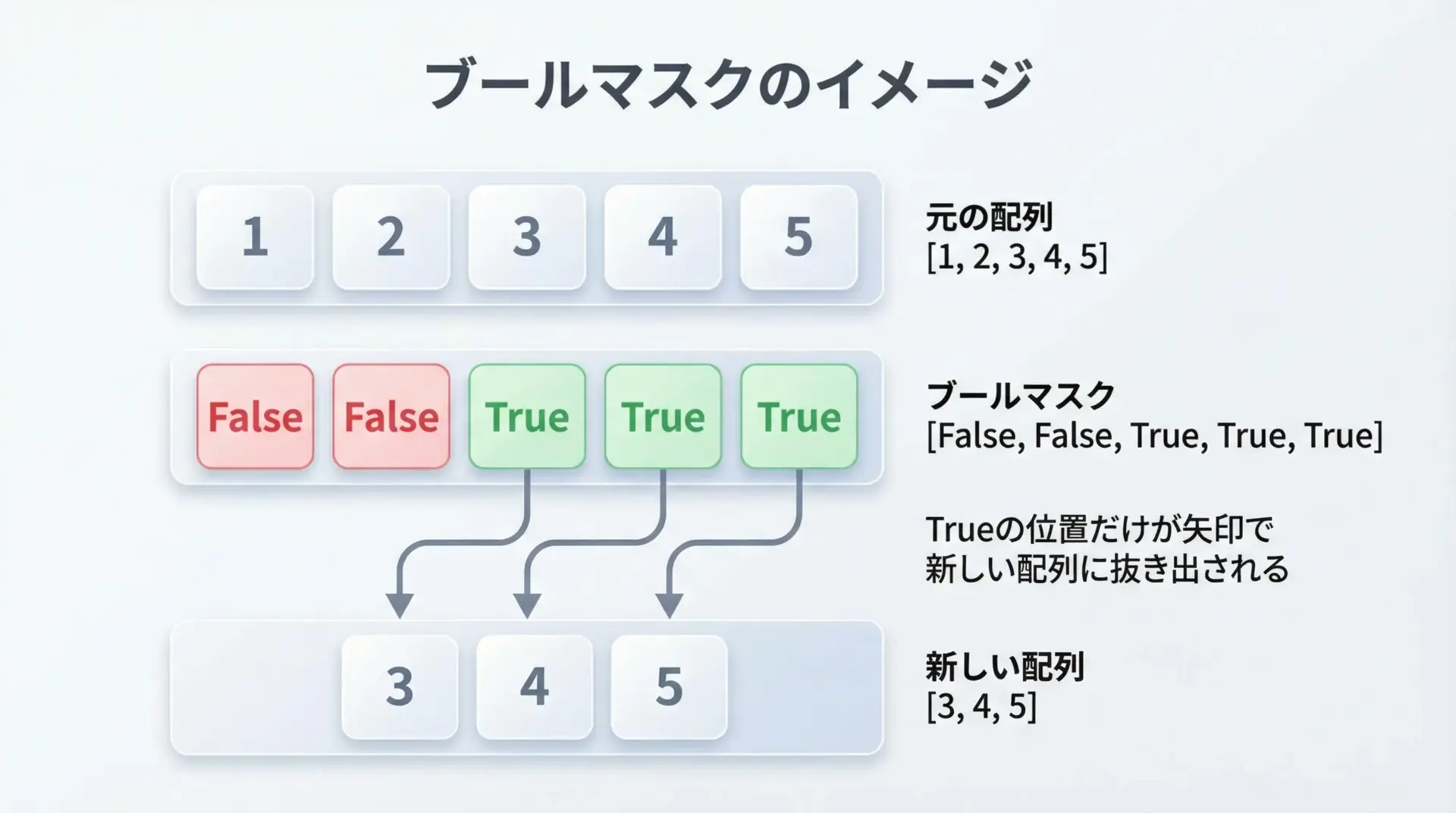
NumPyでは、条件式から得られるブール配列をインデックスとして使うことができます。
これをブールインデックス(ブールマスク)と呼びます。
import numpy as np

arr = np.array([1, 2, 3, 4, 5, 6])

# 条件に合致する要素だけを抽出
mask = arr > 3
result = arr[mask]

print("元配列:", arr)
print("マスク:", mask)
print("3より大きい要素:", result)元配列: [1 2 3 4 5 6]
マスク: [False False False True True True]
3より大きい要素: [4 5 6]ブールインデックスを使うことで、forループやif文を書かずに条件抽出ができるため、コードが簡潔かつ高速になります。
高次元配列のインデックス指定
3次元以上の場合も、同じようにカンマ区切りでインデックスを指定します。
import numpy as np

# 2×3×4 の3次元配列を作成
arr3d = np.arange(24).reshape(2, 3, 4)

print("3次元配列のshape:", arr3d.shape)
print("0番目のブロック:\n", arr3d[0])
print("1番目ブロックの2行目:\n", arr3d[1, 1])
print("全ブロックの1行目の2列目:", arr3d[:, 0, 1])3次元配列のshape: (2, 3, 4)
0番目のブロック:
[[0 1 2 3]
[4 5 6 7]
[8 9 10 11]]
1番目ブロックの2行目:
[[12 13 14 15]
[16 17 18 19]
[20 21 22 23]]
全ブロックの1行目の2列目: [ 1 13]高次元配列では、どの次元が「高さ」「行」「列」に対応するかを常に意識すると、インデックス指定の誤りを減らせます。
NumPy配列の形状操作
reshapeで配列の形を変える

reshapeは、配列の中身はそのままに、見かけ上の形状だけを変更する関数です。
import numpy as np

arr = np.arange(12)  # 0〜11
print("元配列:", arr)

mat_3x4 = arr.reshape(3, 4)
mat_2x6 = arr.reshape(2, 6)

print("3×4配列:\n", mat_3x4)
print("2×6配列:\n", mat_2x6)元配列: [ 0 1 2 3 4 5 6 7 8 9 10 11]
3×4配列:
[[ 0 1 2 3]
[ 4 5 6 7]
[ 8 9 10 11]]
2×6配列:
[[ 0 1 2 3 4 5]
[ 6 7 8 9 10 11]]いずれの場合も、総要素数は12で等しい必要があります。
また、-1を指定すると、残りの次元を自動計算させることができます。
arr = np.arange(12)

auto = arr.reshape(3, -1)  # 3行?列 → 列数を自動決定
print("3行×自動列:\n", auto)3行×自動列:
[[ 0 1 2 3]
[ 4 5 6 7]
[ 8 9 10 11]]transposeとswapaxesで軸を入れ替える
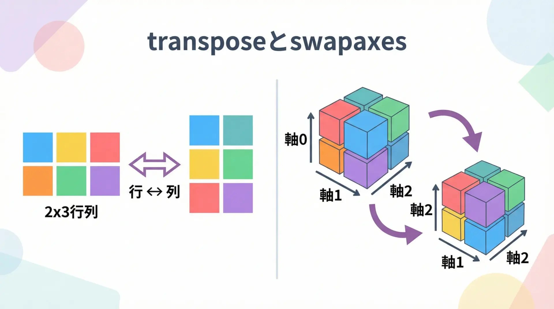
行と列を入れ替える転置は、transposeまたは.T属性で行います。
import numpy as np

mat = np.array([[1, 2, 3],
                [4, 5, 6]])

print("元の行列:\n", mat)
print("転置(メソッド):\n", mat.transpose())
print("転置(属性T):\n", mat.T)元の行列:
[[1 2 3]
[4 5 6]]
転置(メソッド):
[[1 4]
[2 5]
[3 6]]
転置(属性T):
[[1 4]
[2 5]
[3 6]]3次元以上で特定の軸だけを入れ替えたい場合はnp.swapaxesを使います。
import numpy as np

arr = np.zeros((2, 3, 4))  # shape = (2, 3, 4)

# 軸1と2を入れ替える → shape = (2, 4, 3)
swapped = np.swapaxes(arr, 1, 2)

print("元shape:", arr.shape)
print("swapaxes後shape:", swapped.shape)元shape: (2, 3, 4)
swapaxes後shape: (2, 4, 3)flattenとravelで配列を一次元化する
配列を一次元ベクトルに変換するには、flattenまたはravelを使います。
ただし、メモリコピーの有無という重要な違いがあるため注意が必要です。
import numpy as np

mat = np.array([[1, 2],
                [3, 4]])

flat1 = mat.flatten()  # 常にコピーを返す
flat2 = mat.ravel()    # 可能ならビュー(参照)を返す

print("元:\n", mat)
print("flatten:", flat1)
print("ravel :", flat2)元:
[[1 2]
[3 4]]
flatten: [1 2 3 4]
ravel : [1 2 3 4]ravelの戻り値を変更すると、元配列に影響する場合があります。
この挙動を理解しながら、メモリ効率と安全性のバランスを取ることが大切です。
NumPyの基本演算とブロードキャスト
要素ごとの四則演算と比較演算
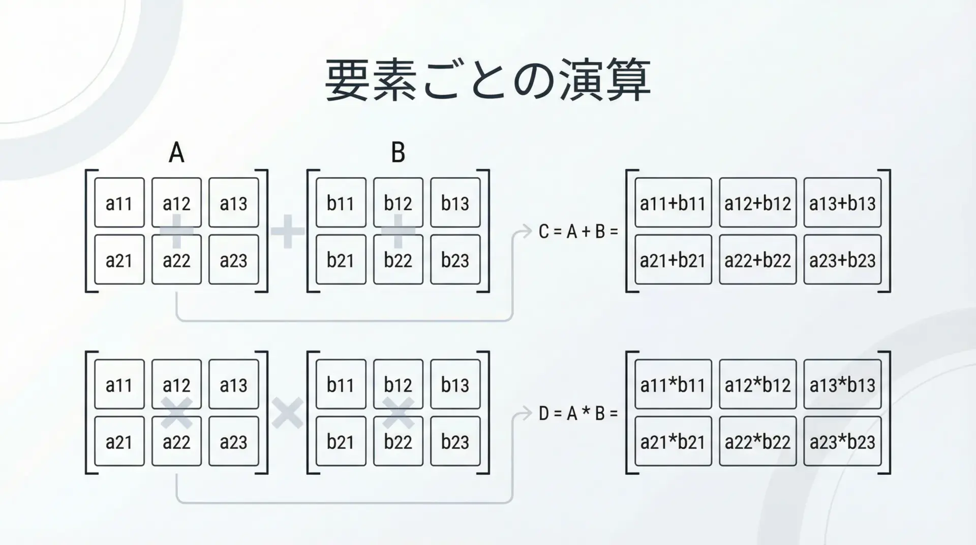
NumPy配列同士の演算は、基本的に要素ごと(element-wise)に行われます。
import numpy as np

a = np.array([1, 2, 3])
b = np.array([10, 20, 30])

print("足し算:", a + b)
print("引き算:", a - b)
print("掛け算:", a * b)
print("割り算:", a / b)
print("比較 (>10):", b > 10)足し算: [11 22 33]
引き算: [-9 -18 -27]
掛け算: [10 40 90]
割り算: [0.1 0.1 0.1]
比較 (>10): [False True True]比較演算の結果はブール配列になります。
これをそのままブールマスクとして利用できるため、条件抽出との相性がとても良いです。
ブロードキャストの仕組みとルール
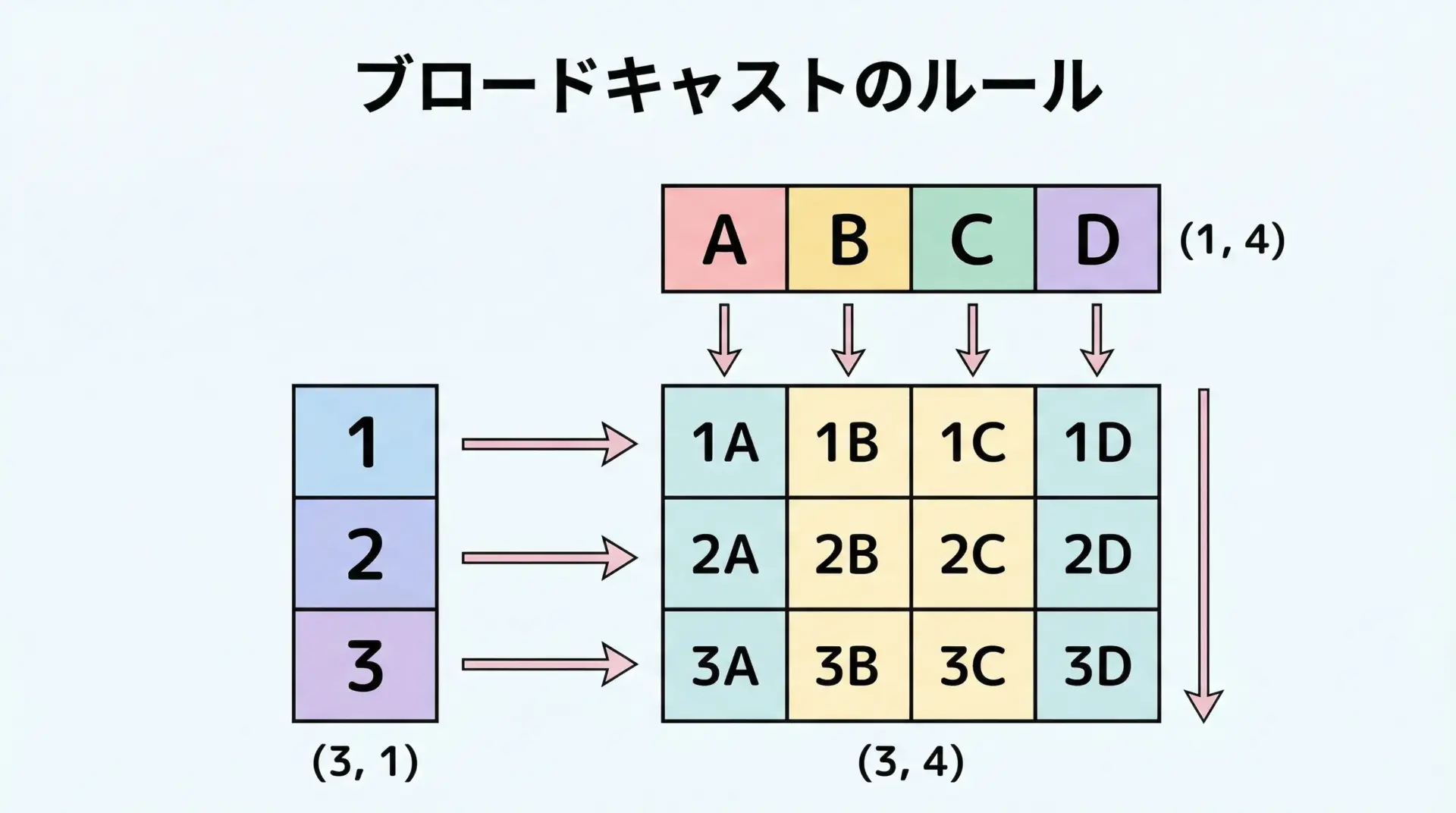
ブロードキャストとは、形状の異なる配列同士でも、特定のルールのもとで自動的に次元を合わせて演算する仕組みです。
代表的な例を見てみます。
import numpy as np

a = np.array([[1, 2, 3],
              [4, 5, 6]])   # shape (2, 3)

b = np.array([10, 20, 30])  # shape (3,)

c = a + b   # bが(1, 3)に広がって足し合わされる

print("aのshape:", a.shape)
print("bのshape:", b.shape)
print("結果:\n", c)aのshape: (2, 3)
bのshape: (3,)
結果:
[[11 22 33]
[14 25 36]]NumPyのブロードキャストには、次のような基本ルールがあります。
- 右端の次元から比較し、同じかどちらかが1ならば「互換性あり」
- 互換性のある次元は、それぞれのサイズの最大値に拡張される
- どの次元でも互換性がない場合はエラーになる
このルールを理解しておくと、後述するブロードキャストエラーの原因も見通しやすくなります。
スカラー演算と配列演算の違い
スカラー(単一の数値)と配列を演算すると、スカラーが配列全体にブロードキャストされます。
import numpy as np

arr = np.array([1, 2, 3])

print("全要素に10を足す:", arr + 10)
print("全要素を2倍:", arr * 2)全要素に10を足す: [11 12 13]
全要素を2倍: [2 4 6]このように、スカラー演算は暗黙に「全要素に対する一括処理」になっているため、非常に直感的です。
forループを書く必要はありません。
集約関数と統計量の計算
sum・mean・stdなどの基本集約関数
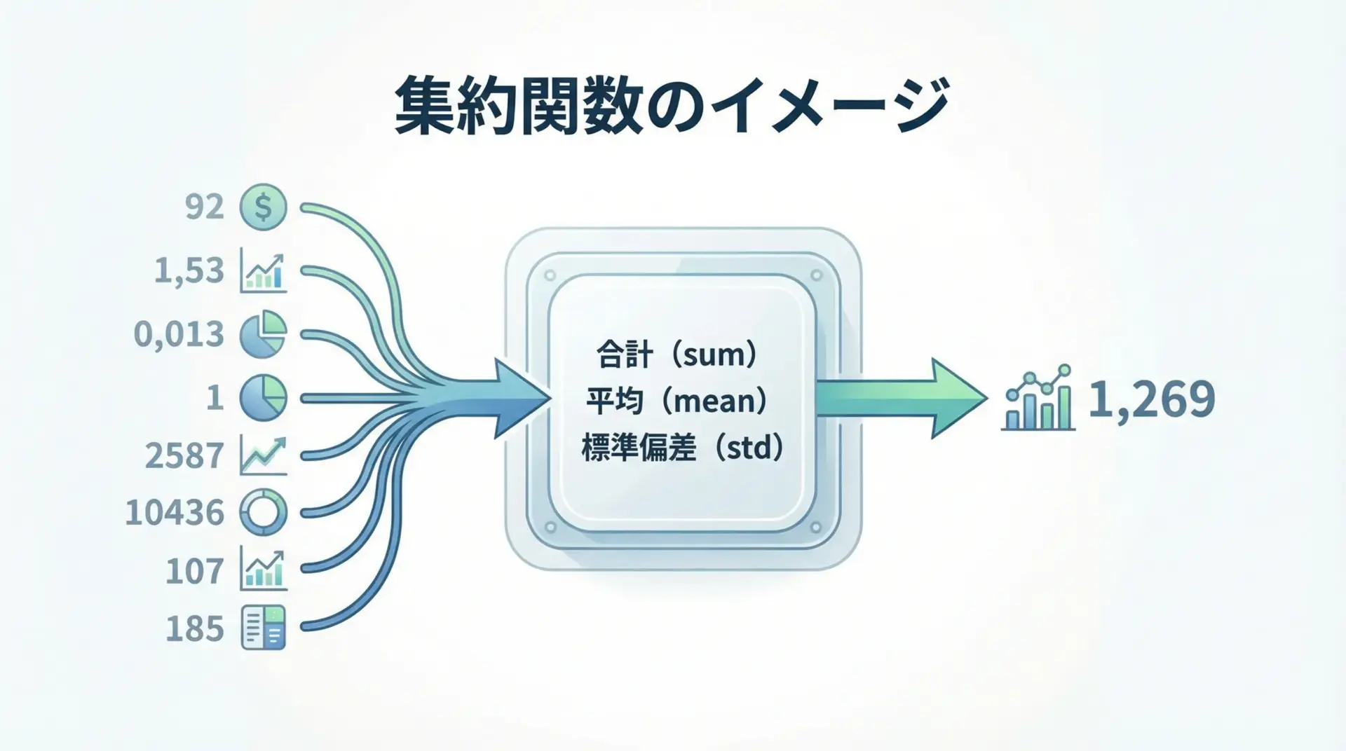
NumPyには、配列から単一の値を計算する集約(集計)関数が豊富に用意されています。
import numpy as np

arr = np.array([1, 2, 3, 4, 5])

print("合計:", arr.sum())
print("平均:", arr.mean())
print("標準偏差:", arr.std())
print("分散:", arr.var())合計: 15
平均: 3.0
標準偏差: 1.4142135623730951
分散: 2.0これらの関数はメソッドとしても、np.sum(arr)のような関数形式としても呼び出せます。
axisを指定した行方向・列方向の集計

2次元以上では、axis引数でどの方向に集約するかを指定できます。
import numpy as np

mat = np.array([[1, 2, 3],
                [4, 5, 6]])

print("全要素の合計:", mat.sum())
print("列ごとの合計(axis=0):", mat.sum(axis=0))
print("行ごとの合計(axis=1):", mat.sum(axis=1))全要素の合計: 21
列ごとの合計(axis=0): [5 7 9]
行ごとの合計(axis=1): [ 6 15]axis=0は「縦方向(行方向)に潰して列ごとに集計」、axis=1は「横方向(列方向)に潰して行ごとに集計」と覚えておくと理解しやすいです。
max・min・argmax・argminの使い方
最大値・最小値と、それが現れるインデックスを求める関数もよく使います。
import numpy as np

arr = np.array([10, 3, 7, 15, 9])

print("最大値:", arr.max())
print("最小値:", arr.min())
print("最大値の位置(argmax):", arr.argmax())
print("最小値の位置(argmin):", arr.argmin())最大値: 15
最小値: 3
最大値の位置(argmax): 3
最小値の位置(argmin): 12次元以上でも、axisを指定して行・列ごとの最大値を求めることができます。
高速な線形代数処理
dotとmatmulで行列積を計算する

行列積(線形代数でいう行列同士の掛け算)は、np.dotや@演算子、np.matmulで計算します。
import numpy as np

A = np.array([[1, 2, 3],
              [4, 5, 6]])      # shape (2, 3)

B = np.array([[1, 2],
              [3, 4],
              [5, 6]])         # shape (3, 2)

C1 = np.dot(A, B)   # 関数
C2 = A @ B          # 演算子 (Python 3.5+)

print("行列積C1:\n", C1)
print("行列積C2:\n", C2)行列積C1:
[[22 28]
[49 64]]
行列積C2:
[[22 28]
[49 64]]要素ごとの掛け算と行列積は完全に別物なので、用途に応じて使い分ける必要があります。
転置・逆行列・行列式の基本
線形代数では、転置行列、逆行列、行列式などの操作がよく登場します。
NumPyではnp.linalgモジュールがこれらを提供します。
import numpy as np

A = np.array([[1, 2],
              [3, 4]])

# 転置
AT = A.T

# 逆行列
A_inv = np.linalg.inv(A)

# 行列式
det = np.linalg.det(A)

print("A:\n", A)
print("Aの転置:\n", AT)
print("Aの逆行列:\n", A_inv)
print("Aの行列式:", det)A:
[[1 2]
[3 4]]
Aの転置:
[[1 3]
[2 4]]
Aの逆行列:
[[-2. 1. ]
[ 1.5 -0.5]]
Aの行列式: -2.0000000000000004逆行列は正方行列かつ行列式が0でない場合にしか存在しません。
データ分析の実務では、数値誤差や特異行列の問題から、逆行列を直接求めるのではなく、後述する線形方程式として解く方が安定です。
線形方程式をNumPyで解く方法
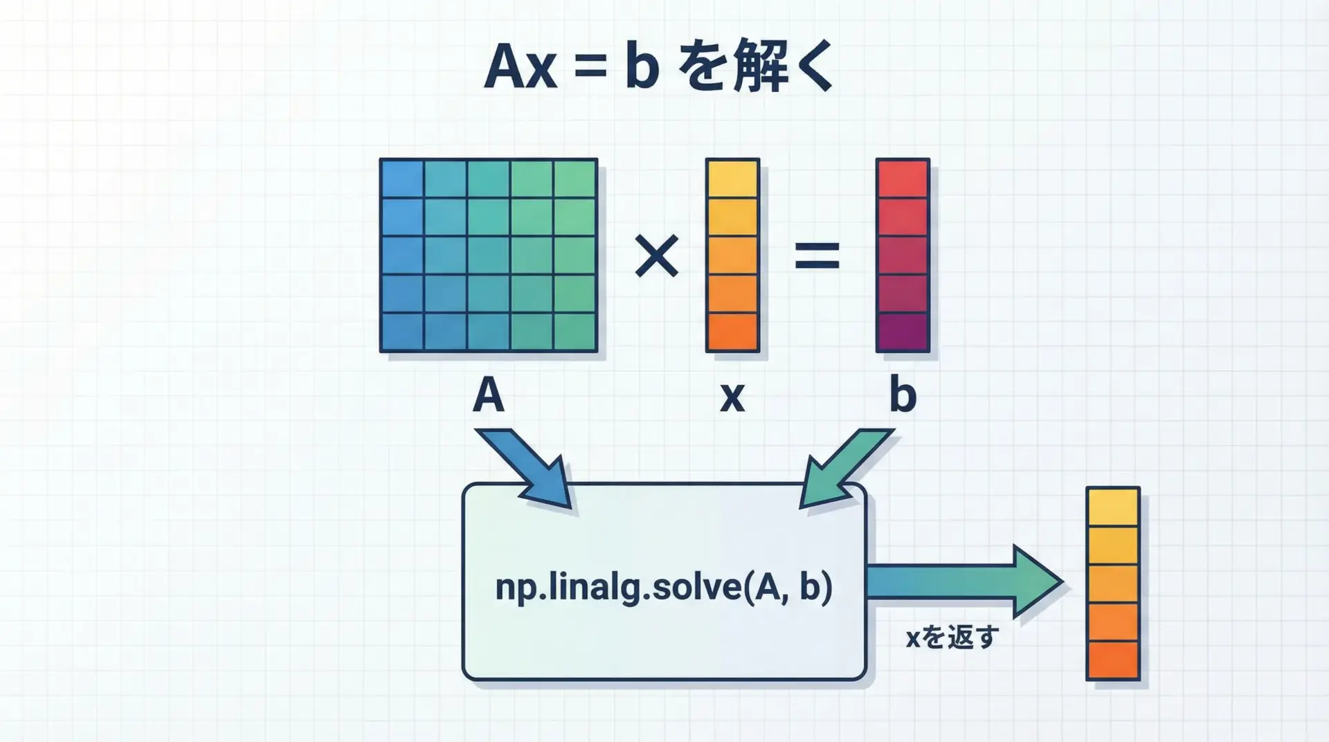
線形方程式Ax = bを解くには、np.linalg.solveを用います。
import numpy as np

# 2つの変数 x, y について
# 2x + y = 1
# x  - y = 0  を解く
A = np.array([[2, 1],
              [1, -1]])
b = np.array([1, 0])

x = np.linalg.solve(A, b)

print("解 x, y:", x)解 x, y: [0.33333333 0.33333333]これは、逆行列を明示的に計算するよりも数値的に安定で、高速です。
機械学習の回帰分析などでも、内部的には同様の線形代数が多用されています。
NumPyによる高速化テクニック
ベクトル化でforループを排除する

Pythonの純粋なforループは遅いため、大量のデータ処理ではボトルネックになりがちです。
NumPyを使うことで、処理をベクトル化し、forループをNumPy内部(C実装)に押し込めることが重要です。
import numpy as np
import time

# 100万要素
n = 1_000_000
arr = np.random.rand(n)

# Pythonのforループで2乗
start = time.time()
result_py = [x * x for x in arr]
t_py = time.time() - start

# NumPyのベクトル化で2乗
start = time.time()
result_np = arr * arr
t_np = time.time() - start

print("Pythonループの時間:", t_py)
print("NumPyベクトル化の時間:", t_np)Pythonループの時間: 0.0x〜0.1x 秒程度
NumPyベクトル化の時間: 0.00x 秒程度環境にもよりますが、NumPyの方が桁違いに速くなることが多いです。
この差が、NumPyがデータ分析分野で広く使われる理由の一つです。
ブールマスクで条件分岐を高速化
if文を多用する処理も、ブールマスクに置き換えることで高速化できます。
import numpy as np

arr = np.arange(10)

# Pythonループ + if
res_py = []
for x in arr:
    if x % 2 == 0:
        res_py.append(x)

# NumPyのブールマスク
mask = (arr % 2 == 0)
res_np = arr[mask]

print("偶数(ループ):", res_py)
print("偶数(NumPy):", res_np)偶数(ループ): [0, 2, 4, 6, 8]
偶数(NumPy): [0 2 4 6 8]NumPy版は内部でCレベルのループが回るため、Pythonループに比べて高速に動作します。
Pythonループとの速度比較のポイント
速度比較を行う際には、次の点に注意します。
まず、配列のサイズが十分大きくないと、NumPy呼び出しのオーバーヘッドが相対的に大きく見えてしまうことがあります。
また、Jupyter Notebookなどでは最初の実行時にモジュール読み込みが発生するため、何度か繰り返して平均を取るとより公平な比較になります。
さらに、Pythonループ内でNumPy関数を1要素ずつ呼び出すようなパターンは、最悪の組み合わせです。
あくまで、「できるだけ大きな配列に対して一度に処理を行う」ことが高速化の鍵です。
NumPyとブロードキャストを使った実用例
正規化や標準化をNumPyで実装する
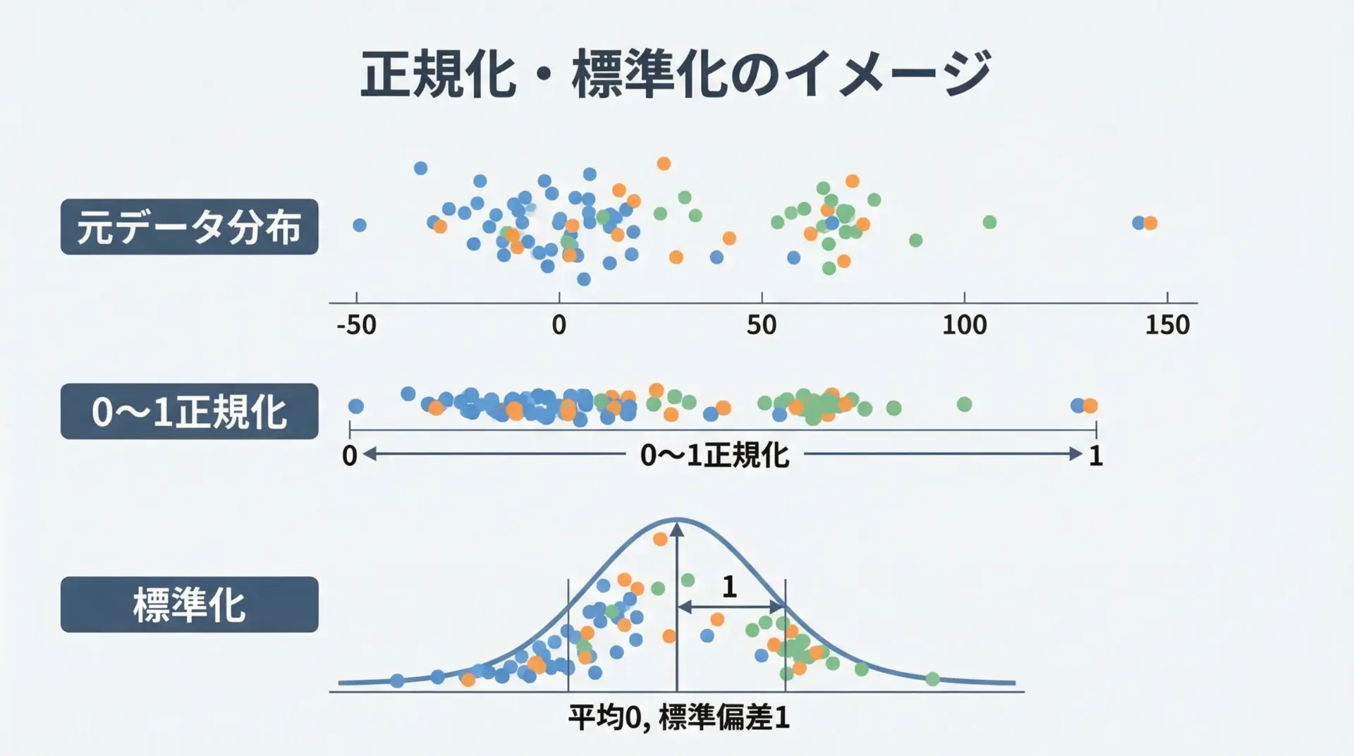
データ前処理でよく使われるのが、正規化(0〜1スケーリング)や標準化(平均0, 標準偏差1)です。
NumPyを使うと、ブロードキャストを活かして簡潔に実装できます。
import numpy as np

X = np.array([[1.0, 10.0, 100.0],
              [2.0, 20.0, 200.0],
              [3.0, 30.0, 300.0]])

# 列ごと(特徴量ごと)に0〜1正規化
X_min = X.min(axis=0)
X_max = X.max(axis=0)
X_norm = (X - X_min) / (X_max - X_min)

print("0〜1正規化:\n", X_norm)

# 列ごとに標準化
X_mean = X.mean(axis=0)
X_std = X.std(axis=0)
X_stdzd = (X - X_mean) / X_std

print("標準化:\n", X_stdzd)0〜1正規化:
[[0. 0. 0. ]
[0.5 0.5 0.5]
[1. 1. 1. ]]
標準化:
[[-1.22474487 -1.22474487 -1.22474487]
[ 0. 0. 0. ]
[ 1.22474487 1.22474487 1.22474487]]このコードでは、X_minやX_meanが(3,)の1次元配列として計算され、それが(3, 3)のXにブロードキャストされて列ごとの演算が実現しています。
距離計算や類似度計算のベクトル化
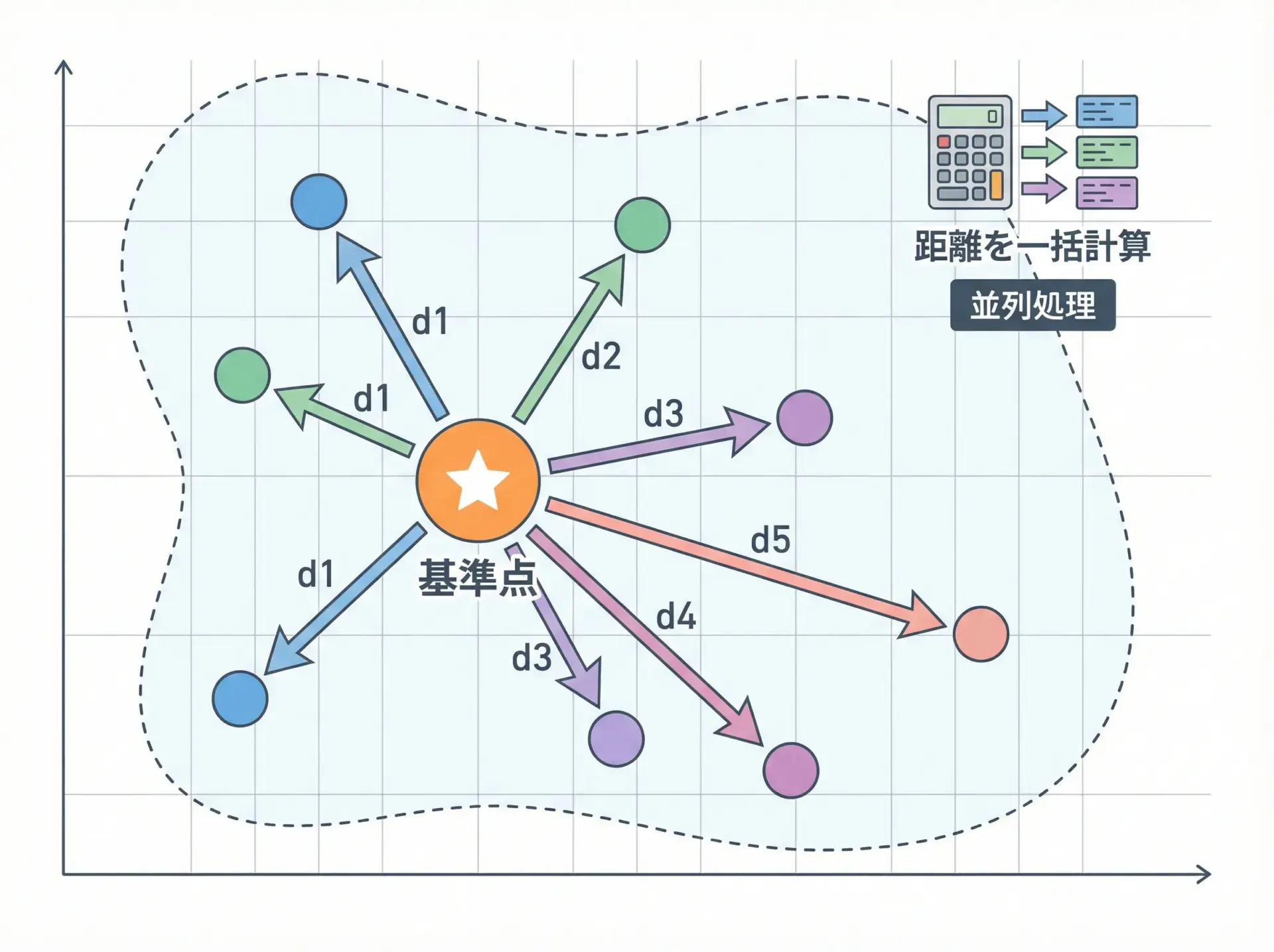
データ分析では、サンプル間の距離や類似度を計算する場面が頻出します。
2つの行列X(n×d)とY(m×d)の全組み合わせのユークリッド距離を、ブロードキャストで計算する例を示します。
import numpy as np

# 3サンプル、2次元
X = np.array([[0, 0],
              [1, 0],
              [0, 1]])

# 2サンプル、2次元
Y = np.array([[1, 1],
              [2, 2]])

# Xを (3, 1, 2)、Yを (1, 2, 2) に拡張して差をとる
diff = X[:, np.newaxis, :] - Y[np.newaxis, :, :]  # shape (3, 2, 2)

# ユークリッド距離
dists = np.sqrt((diff ** 2).sum(axis=2))  # shape (3, 2)

print("距離行列:\n", dists)距離行列:
[[1.41421356 2.82842712]
[1. 2.23606798]
[1. 2.23606798]forループを使うと二重ループが必要な処理も、ブロードキャストを組み合わせれば1〜2行で表現できます。
画像処理における配列操作の例
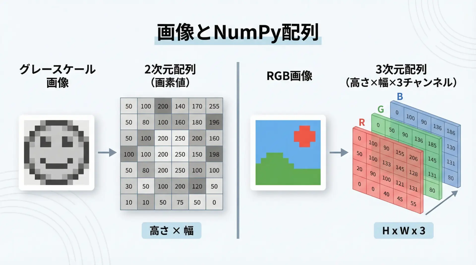
画像はNumPy配列と非常に相性がよいデータ構造です。
例えば、画像の輝度を半分にする処理は次のように書けます。
import numpy as np

# 仮のグレースケール画像(0〜255)
img = np.array([[100, 150],
                [200, 250]], dtype=np.uint8)

# 輝度を半分に(オーバーフローを避けるため一度floatに変換)
img_half = (img.astype(np.float32) / 2).astype(np.uint8)

print("元画像:\n", img)
print("輝度半分:\n", img_half)元画像:
[[100 150]
[200 250]]
輝度半分:
[[50 75]
[100 125]]カラー画像(RGB)なら(高さ, 幅, 3)の3次元配列として表現され、各チャンネルをまとめて操作したり、特定チャンネルだけを抜き出すことも簡単です。
NumPyと他ライブラリとの連携
NumPyとPandasのデータ受け渡し
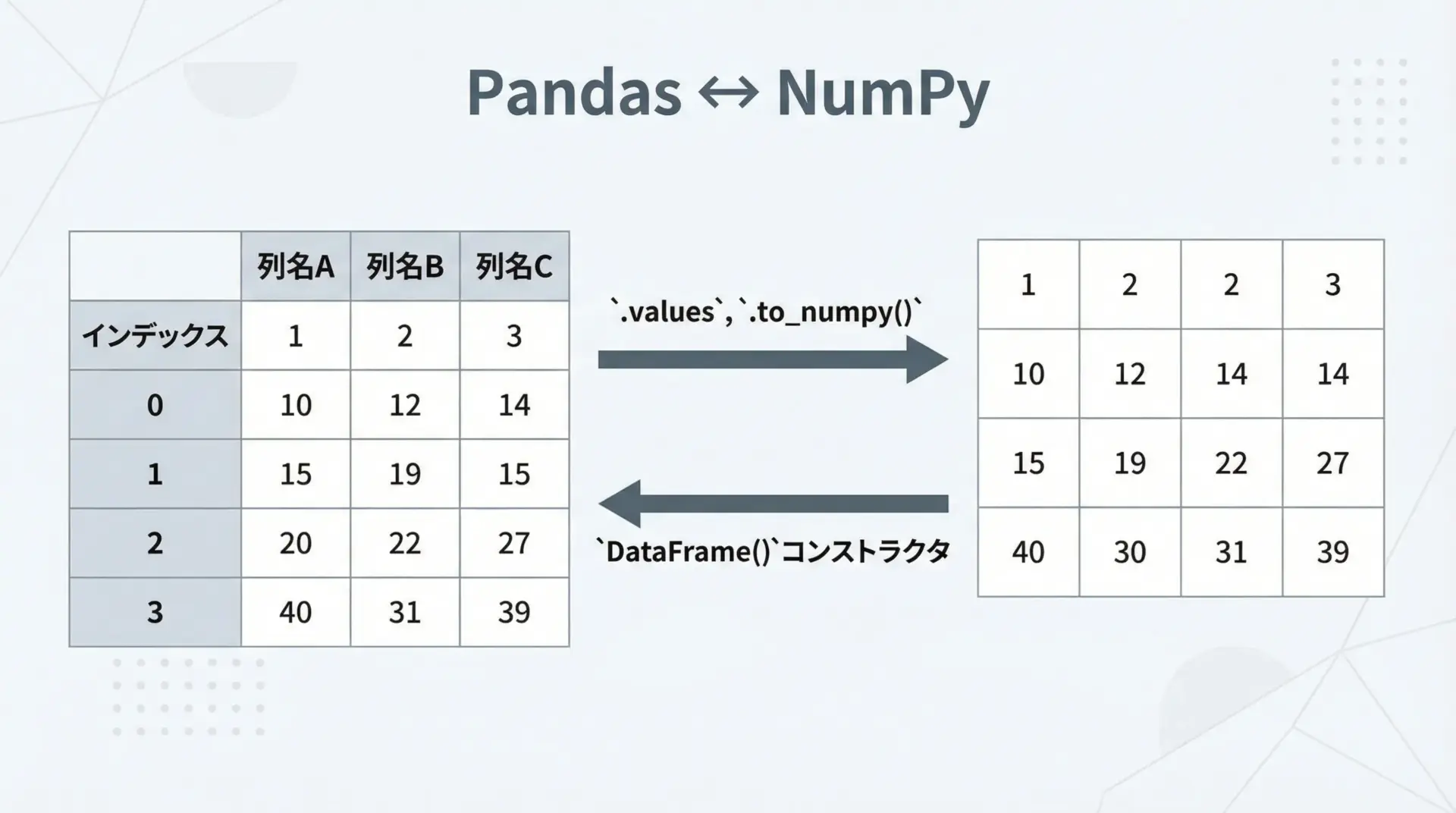
Pandasは内部的にNumPy配列を利用しており、両者のデータ受け渡しは非常にスムーズです。
import numpy as np
import pandas as pd

# NumPy → Pandas
arr = np.array([[1, 2],
                [3, 4]])
df = pd.DataFrame(arr, columns=["A", "B"])
print("DataFrame:\n", df)

# Pandas → NumPy
back_to_np = df.to_numpy()
print("NumPy配列:\n", back_to_np)DataFrame:
A B
0 1 2
1 3 4
NumPy配列:
[[1 2]
[3 4]]機械学習モデルの入力はNumPy配列、特徴量エンジニアリングはPandasで、という使い分けもよく行われます。
NumPyとMatplotlibで可視化する

Matplotlibは、NumPy配列を直接受け取ってグラフを描画するライブラリです。
import numpy as np
import matplotlib.pyplot as plt

# 0〜2πまでを100点に分割
x = np.linspace(0, 2 * np.pi, 100)
y = np.sin(x)

plt.plot(x, y, label="sin(x)")
plt.xlabel("x")
plt.ylabel("sin(x)")
plt.legend()
plt.title("Sine wave")
plt.show()(グラフウィンドウにサイン波が表示されます)NumPyでデータを計算し、Matplotlibで可視化するという流れは、データサイエンスの基本パターンです。
SciPyとNumPyの関係と使い分け
SciPyは、NumPyを土台としたより高水準な科学技術計算ライブラリです。
NumPyが配列と基本演算を提供するのに対し、SciPyは数値積分、最適化、信号処理、統計、疎行列など、専門的なアルゴリズムを多数実装しています。
実務では、次のような役割分担になることが多いです。
- NumPy: 配列操作、線形代数の基礎、統計量の簡易計算
- SciPy: 複雑な最適化問題、微分方程式、信号処理、より高度な統計検定
いずれもNumPy配列を共通フォーマットとして扱うため、シームレスに連携できます。
NumPyの型(dtype)とメモリ効率
dtypeの種類と選び方
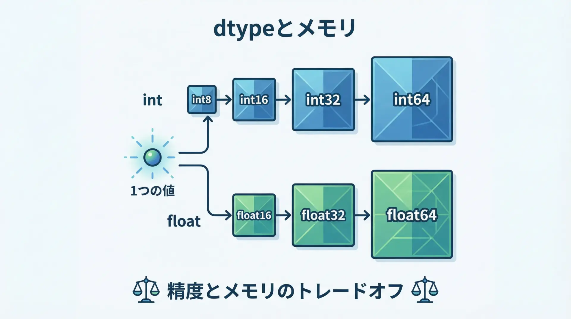
NumPy配列は、すべての要素が同じデータ型(dtype)であるという特徴があります。
代表的なdtypeには次のようなものがあります。
- 整数:
int8,int16,int32,int64 - 浮動小数点:
float16,float32,float64 - 真偽値:
bool
import numpy as np

arr_int = np.array([1, 2, 3], dtype=np.int32)
arr_float = np.array([1, 2, 3], dtype=np.float64)

print("int32 dtype:", arr_int.dtype)
print("float64 dtype:", arr_float.dtype)int32 dtype: int32
float64 dtype: float64精度が高いdtypeほどメモリ消費が大きく計算も重くなるため、用途に応じて適切な型を選ぶことが重要です。
astypeで型変換する方法
dtypeを変更したい場合は、astypeメソッドを使います。
import numpy as np

arr = np.array([1.1, 2.5, 3.9])
print("元dtype:", arr.dtype)

# 整数に変換(小数点以下切り捨て)
arr_int = arr.astype(np.int32)
print("変換後dtype:", arr_int.dtype)
print("変換後値:", arr_int)元dtype: float64
変換後dtype: int32
変換後値: [1 2 3]astypeは基本的に新しい配列を返し、元配列を変更しない点に注意してください。
大規模データでは、このコピーコストも無視できないことがあります。
大規模データでのメモリ節約テクニック

大規模データを扱う場合、dtype選びはメモリ使用量に大きく影響します。
例えば、0〜255の画素値しか入らない画像ならuint8で十分ですし、IDのように範囲が限られる整数もint16やint32で足りることが多いです。
import numpy as np

# 1億要素の配列でメモリ消費を比較
n = 100_000_000

a_int64 = np.zeros(n, dtype=np.int64)
a_int16 = np.zeros(n, dtype=np.int16)

print("int64配列のバイト数:", a_int64.nbytes)
print("int16配列のバイト数:", a_int16.nbytes)int64配列のバイト数: 800000000
int16配列のバイト数: 200000000このように、dtypeを適切に選ぶだけでメモリ使用量を何倍も節約できることがあります。
NumPyのよくあるエラーと対処法
shape不一致によるブロードキャストエラー
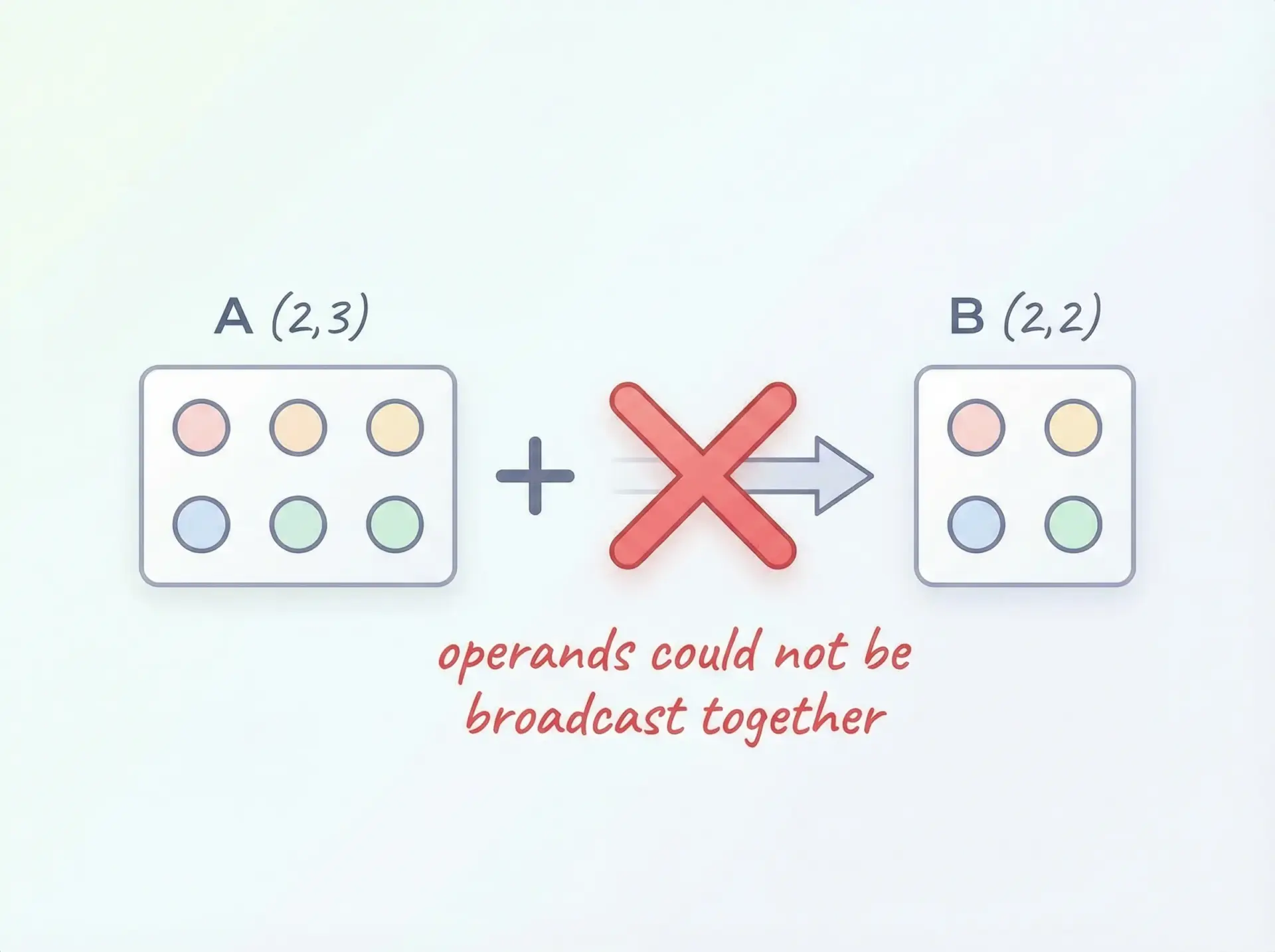
ブロードキャストのルールに合わない配列同士を演算しようとすると、次のようなエラーが出ます。
import numpy as np

a = np.zeros((2, 3))
b = np.zeros((2, 2))

# これはエラーになる
c = a + bValueError: operands could not be broadcast together with shapes (2,3) (2,2)対処法としては、各配列のshapeを確認し、どの次元が不一致かを特定します。
その上で、reshapeやnp.newaxisを用いて、ブロードキャスト可能な形に整形します。
次元不足・次元過多のインデックスエラー
配列の次元数に合わないインデックス指定をすると、エラーになります。
import numpy as np

arr = np.array([1, 2, 3])  # shape = (3,)

# 2次元インデックスでアクセスしようとするとエラー
value = arr[0, 0]IndexError: too many indices for array: array is 1-dimensional, but 2 were indexedこの場合は配列のndimとshapeを確認し、インデックスの数を揃える必要があります。
逆に、np.newaxisを使って次元を増やすことで、意図したインデックス指定を可能にすることもあります。
型変換時の注意点とデバッグ方法
astypeによる型変換では、値の丸めやオーバーフローに注意が必要です。
import numpy as np

arr = np.array([1.9, 2.1], dtype=np.float32)
arr_int = arr.astype(np.int8)

print("元:", arr)
print("変換後:", arr_int)元: [1.9 2.1]
変換後: [1 2]小数点以下は切り捨てられるため、必要であればnp.roundやnp.floorなどで事前に制御します。
また、デバッグ時には次の点を確認すると原因が見つかりやすくなります。
print(arr.dtype, arr.shape)で型と形状を確認- 一時変数を細かく出力して、どの段階で意図しない変換が起きたかを特定
- 小さなサンプルデータで再現性のあるテストを行う
dtypeとshapeを意識的に確認することが、NumPyのトラブルシューティングにおいて最も重要なポイントです。
まとめ
NumPyは、Pythonでの数値計算やデータ分析を支える基盤ライブラリであり、多次元配列ndarrayとブロードキャスト、高速なベクトル化演算を中心に設計されています。
本記事では、インストールから配列生成、インデックス・形状操作、ブロードキャスト、統計量計算、線形代数、実用的な前処理・距離計算、他ライブラリとの連携、dtypeとメモリ効率、そしてよくあるエラーまで一通り解説しました。
日常的にshape・dtype・axisを意識しながらコードを書くことで、NumPyの力を最大限に引き出し、読みやすく高速な数値処理が実現できるようになります。
